CoppeliaSim Introduction

CoppeliaSim Introduction

Note: CoppeliaSim is computationally intensive. To minimize power usage, make sure to "pause" or "stop" a simulation when you are not using it.

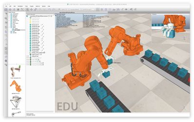
On CoppeliaSim's homepage the program is described as

  ...the Swiss army knife among robot simulators: you won't find a simulator with more functions, features, or more elaborate APIs.

CoppeliaSim's strength comes from several features:

1. CoppeliaSim provides a unified framework combining many powerful internal and external libraries that are often useful for robotics simulations. This includes dynamic simulation engines, forward/inverse kinematics tools, collision detection libraries, vision sensor simulations, path planning, GUI development tools, and built-in models of many common robots.
2. CoppeliaSim is highly extensible. CoppeliaSim developers provide an API that allows one to write custom plugins that add new features. You can embed Lua scripts directly into a simulation scene that, for example, process simulated sensor data, run control algorithms, implement user interfaces, or even send data to a physical robot. They also provide a remote API that allows one to develop standalone applications in many programming languages that are able to pass data in and out of a running CoppeliaSim simulation.
3. CoppeliaSim is cross-platform, mostly open-source, and provides a free educational license.

The purpose of this page is not to teach you how to use CoppeliaSim. Rather it is to describe demonstration scenes that have been developed to support learning from the book Modern Robotics. If you are interested to learn more about CoppeliaSim, check out the Useful Resources section below.

Demonstration V-REP Scenes

DOWNLOAD ALL DEMONSTRATION CoppeliaSim SCENES AND INPUT FILES DESCRIBED BELOW, DATED NOVEMBER 2019.

Older versions of the scenes:

• August 2018

To run any of the scenes below, the first step will be to download CoppeliaSim for your operating system. You should download the latest non-limited EDUCATIONAL version. Next you will have to install CoppeliaSim. On Windows, you simply have an EXE that installs CoppeliaSim. On a Mac, you first need to unzip the download. The directory that is produced by unzipping the download contains a coppeliaSim.app directory that should allow you start coppeliaSim through normal mechanisms, e.g., Finder/Spotlight/Launchpad. On Linux, you will need to extract the compressed tar archive (e.g., using a command like tar xvf CoppeliaSim_Edu_V4_0_0_Ubuntu18_04.tar.xz). Then you need to change directories into the CoppeliaSim source directory and run the coppeliaSim.sh shell script. See this page for more information on getting started with CoppeliaSim.

Once CoppeliaSim is open you will want to run one of the scenes below. To run any of them, you first run CoppeliaSim, then you click File->Open scene... and open one of the ttt files that are linked below. Then click either the Play button from the top toolbar or click Simulation->Start simulation and a GUI should pop up. Clicking the Stop button or Simulation->Stop simulation will close the GUI and stop the simulation.

Most of the scenes feature a simulation of a kinematically-controlled, non-respondable robot. Kinematically controlled means that all dynamics (inertias, torques, friction, etc.) of the system are neglected. We specify a configuration of the robot and it is instantaneously "teleported" to the new configuration. Non-respondable means that the links of the robot are not capable of interacting with the world or each other through collisions. In other words, we can put the robot in configurations that result in self-collisions.

The "interactive" scenes allow you to visualize the robot as you change its configuration using sliders. The "CSV" scenes allow animations of a robot based on a trajectory stored in a comma-separated values file, where each line corresponds to a timestep and consists of comma-separated numbers specifying the robot's configuration at that timestep. There are no joint limits in the "CSV" scenes.

This page has information on writing csv files in Python, MATLAB, and Mathematica.

The CSV mobile manipulation scene is a partly dynamically-controlled simulation of a respondable youBot from KUKA.

Important note regarding csv file format: The example csv files included below for use with the csv scenes assume that periods, not commas, are used as decimal points. So pi is written as 3.14, not as 3,14. If you are using Linux and your region settings are set to a region that uses commas as the decimal separator, one solution, suggested by a Coursera student, is to invoke CoppeliaSim using US English settings:

LC_NUMERIC=en_US.UTF-8 ./coppeliaSim.sh

Another option, also suggested by a Coursera student, is to open the Linux "System Settings" -> "Language support" -> "Regional Formats" tab. After changing the region to "English (United States)", log out and back in for the change to take effect.

In each scene, there is a single Lua script called a non-threaded child script. When the scene is first run, there is a function that is called that sets up the GUI and creates variables that are going to be needed later on in the simulation. Then during every step of the simulation the main script, which is part of every CoppeliaSim scene, runs an "actuation" function from the child script. This actuation function is responsible for processing all of the changes to the GUI since the last time it was called (buttons clicked, label updates, etc.), and for sending joint commands to the simulated robot. Technically, there is also a "sensing" function in the child script that gets called by the main script, but in each of these scenes, the sensing function is empty. The GUIs are all built with CoppeliaSim's Qt-based custom UI framework.

Scene 1: Interactive UR5

(This scene had minor updates in August 2018.)

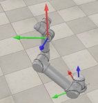
This scene helps you visualize a UR5 robot from Universal Robots. The model of the UR5 was created by importing a URDF from the ROS-Industrial ur5_description package. The GUI in this scene features two tabs. One tab lets you drag sliders to modify the joint angles of each joint, and the other tab allows you to specify comma-separated angles for all 6 joints in an editable text box and ask for the SE(3) transformation from the base frame to the end-effector frame. The frames attached to the base and end-effector are persistently displayed (x-axis in red, y-axis in green, z-axis in blue). Note that all angles are specified in radians.

Scene 1 files in the download of all of the demonstration scenes:

• Scene1_UR5.ttt: the CoppeliaSim scene file.

Scene 2: CSV Animation UR5

(This scene had minor updates in August 2018.)

This scene animates the motion of the UR5 robot based on a csv file representing the trajectory of the robot. Each row of the csv file represents a timestep and each column of the csv file is the joint angle through time for one of the joints (first column is joint 1, last column is joint 6).

Scene 2 files in the download of all of the demonstration scenes:

• Scene2_UR5_csv.ttt: the CoppeliaSim scene file.
• Scene2_example.csv: an example input file.

See the note above about making sure your language settings are appropriate to properly read csv files in Linux.

Scene 3: Interactive youBot

(Updated August 2018, to match the frame conventions used in the textbook and in Scene 4, animation of the youBot.)

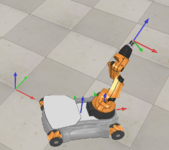
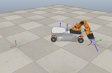
This scene helps you visualize a youBot mobile manipulator from KUKA. The KUKA youBot consists of a mecanum-wheel omnidirectional base and a 5R robot arm. Move the mobile base of the robot and the joints of the robot using sliders, and inspect the SE(3) representation of the resulting end-effector coordinate frame. All angles are represented in radians, and linear distances are represented in meters. The following frames are illustrated: the world frame {s}, a frame fixed to the center of the mobile chassis {b}, a frame fixed at the base of the robot arm {0}, and a frame fixed to the end-effector {e}.

Scene 3 files in the download of all of the demonstration scenes:

• Scene3_youBot.ttt: the CoppeliaSim scene file.

Scene 4: CSV Animation youBot

(This scene had minor updates in August 2018.)

This scene animates the motion of the youBot based on a csv file representing the trajectory of the robot. Each row of the csv file represents a timestep and each column of the csv file is a configuration variable through time. The csv file has either 12 or 13 columns. Columns 1-3 represent the mobile base configuration variables, ordered as (phi, x, y), where phi is the angle of the base and (x, y) is the location of its center. Columns 4-8 represent the five arm joint angles, joint 1 through joint 5. Columns 9-12 represent the wheel angles, where wheel 1 is column 9 and wheel 4 is column 12, and the numbering of the wheels is shown in the figure on the right. Column 13 is optional. If it is present, then 0 means the gripper is open and 1 means the gripper is closed. If there is no column 13, then the gripper is open by default. All angles are specified in radians.

Scene 4 files in the download of all of the demonstration scenes:

• Scene4_youBot_csv.ttt: the CoppeliaSim scene file.
• Scene4_example.csv: an example input file.
• Scene4_base_motions: this folder has five basic motions of the youBot mobile base, showing the correct wheel motions associated with some basic motions of mobile base. You can check that your wheeled mobile base kinematics (or odometry) are correct by comparing your wheel motions to the wheel motions in these .csv files.
  • yb1.csv: Constant speed spin in place (wheels on the left side and right side of the robot move at opposite speeds).
  • yb2.csv: Constant speed forward motion (all wheels move at the same speed).
  • yb3.csv: Constant speed sideways motion (wheels on opposite corners move at the same speed).
  • yb4.csv: Constant speed diagonal motion (wheels 2 and 4 move at the same speed while wheels 1 and 3 are stationary).
  • yb5.csv: Constant speed diagonal motion (wheels 1 and 3 move at the same speed while wheels 2 and 4 are stationary).

See the note above about making sure your language settings are appropriate to properly read csv files in Linux.

Scene 5: CSV Motion Planning Kilobot

(This scene had minor updates in August 2018.)

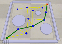
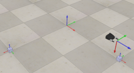
This scene allows you to visualize motion planning on an undirected graph using graph-search techniques such as A*. To visualize the planned motion, we are using the kilobot robot moving in a planar square environment of dimensions -0.5 <= x <= 0.5 and -0.5 <= y <= 0.5. Obstacles are represented as cylinders, and the graph itself is illustrated as blue nodes with yellow edges. The path that the kilobot actually follows is indicated by green edges, and the goal node is in red. See the image to the right.

This scene does not do motion planning. Instead, it displays the output of your motion planner. It expects you to provide the path to a folder with four files, named nodes.csv, edges.csv, path.csv, and obstacles.csv:

• nodes.csv: If the graph has N nodes, then this file has N rows. Each row is of the form ID,x,y,heuristic-cost-to-go. ID is the unique integer ID number of the node, and these ID numbers should take values 1 through N. x, y are the (x,y) coordinates of the node in the plane. heuristic-cost-to-go is an optimistic approximation of the shortest path from this node to the goal node (e.g., the Euclidean distance to the goal node). This information is useful for A-star search but is not represented in the visualization of the path.

• edges.csv: If the graph has E edges, then this file has E rows. Each row is of the form ID1,ID2,cost. ID1 and ID2 are the node IDs of the nodes connected by the edge. cost is the cost of traversing that edge. This file can be empty if you do not wish to display edges.

• path.csv: This file specifies the solution path in the graph, and it is a single line, of the form ID1,ID2,... The first number is the ID of the first node in the solution path, and the last number is the ID of the last node in the solution path. If there is no solution to the motion planning problem, the path can consist of a single ID number, the ID of the node where the robot starts (and stays).

• obstacles.csv: This file specifies the locations and diameters of the circular obstacles. Each row is x, y, diameter, where (x,y) is the center of the obstacle and diameter is the diameter of the obstacle. This file can be empty if there are no obstacles.

Nothing prevents you from providing files with nodes or edges inside obstacles. The path.csv file is the output of a graph search planner. Inputs to the planner could be the obstacles.csv file and a specification of the positions of the start and goal nodes, or it could be the nodes.csv and edges.csv files and a specification of the start and goal nodes, or it could be other information, depending on your planner. But in any case, this scene requires the four files above for the visualization.

Scene 5 files in the download of all of the demonstration scenes:

• Scene5_motion_planning.ttt: the CoppeliaSim scene file.
• Scene5_example.zip: a directory containing example input files nodes.csv, edges.csv, path.csv, and obstacles.csv.

See the note above about making sure your language settings are appropriate to properly read csv files in Linux.

You may be interested in:

• A description of an A* search project using this scene.
• A description of a sampling-based planning project using this scene.

Scene 6: CSV Mobile Manipulation youBot

(This scene had minor updates in November 2019, to fix a problem on some Macs in loading csv files.)

This page has a description of a capstone mobile manipulation project using this scene, as well as more details regarding the operation of the physics engines, the kinematics of the youBot, properties of the end-effector (gripper), and properties of the cube.

This scene has a youBot mobile manipulator and a cube. The youBot is expected to pick up the cube and put it down at a goal location ("pick and place"). This scene animates a user-specified csv file specifying the motion of the youBot, much as in Scene 4, except now the gripper interacts dynamically with the cube. Each row of the csv file has 13 variables: 3 for the chassis configuration (phi, x, y), 5 for the arm joint angles, 4 for the wheel angles (where the wheels are numbered as shown in Scene 4), and 1 for the gripper state (0 = open, 1 = closed). Unlike previous csv visualization scenes where CoppeliaSim simply makes a movie of the configurations, and there is no notion of the simulated time between successive lines in the csv file, this CoppeliaSim scene is performing a dynamic simulation, so the time between each line is important to determine the dynamic behavior. The simulated time between each line of the csv file is 0.01 seconds (10 milliseconds).

The gripper of the youBot and the cube are dynamically modeled to simulate practical pick-and-place. In other words, if the gripper does not close on the block properly, it may slide away, and if you open the gripper when it is holding a block, the block will fall to the floor. The interaction between the gripper and the block is governed by a "physics engine," which approximately accounts for friction, mass, inertial, and other properties. The default physics engine for this scene is ODE.

Gripper opening and closing may take up to approximately 0.625 seconds. Assume, for example, that the first 100 lines of your csv file have the gripper state as 0 (open). Then, on line 101, you change the gripper state to 1 (closed). This transition from 0 to 1 initiates the closing action, but the closing may not actually complete for 0.625 seconds. So you should keep the gripper state at 1 for at least 63 consecutive lines of your csv file to ensure that the gripper closes all the way. Similarly, it may take up to 0.625 seconds for the gripper to open, so you should keep the gripper state at 0 for at least 63 consecutive lines to ensure that the gripper opens all the way. Gripper opening/closing actually terminates when a force threshold is reached on the fingers or the fingers have completed the motion.

You can set the initial and goal configurations of the cube with a GUI inside the scene, but the default initial configuration is $(x,y,\theta )=(1~{\text{m}},0~{\text{m}},0~{\text{rad}})$ and the goal configuration is at $(x,y,\theta )=(0~{\text{m}},-1~{\text{m}},-\pi /2~{\text{rad}})$.

Scene 6 files in the download of all of the demonstration scenes:

• Scene6_youbot_cube.ttt: the CoppeliaSim scene file.
• Scene6_example.csv: an example input file solving the task when the cube's initial and goal configurations are the defaults.

See the note above about making sure your language settings are appropriate to properly read csv files in Linux.

Scene 7: CSV Animation MTB

(This scene had minor updates in August 2018.)

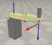
This scene simulates a RRPR robot. It animates a csv file containing a trajectory of joint angles. Each column of the csv file is the joint angle/length through time for one of the joints (in the order of RRPR). A single row of the csv file represents a complete configuration of the robot at a particular time. The prismatic joint (P) has the joint limit range [0, 0.2]. The assumed time step between rows is equal to the time step that CoppeliaSim uses for simulation; the default is 0.05 seconds.

Scene 7 files in the download of all of the demonstration scenes:

• Scene7_MTB_csv.ttt: the CoppeliaSim scene file.
• Scene7_example.csv: An example input file.

See the note above about making sure your language settings are appropriate to properly read csv files in Linux.

Scene 8: CSV youBot End-Effector Animation

(This scene had minor updates in August 2018.)

This page has a description of a capstone mobile manipulation project (specifically Milestone 2) using this scene.

This scene is used in Milestone 2 of the capstone mobile manipulation project. It animates the motion of the gripper of the youBot only (the rest of the youBot is not shown), and this scene is used to validate the planned motion of the gripper. Each line of the csv file has 13 comma-separated values: 12 from the top three rows of the transformation matrix $T_{se}$ representing the configuration of the end-effector frame {e} relative to the space frame {s}, and 1 representing the gripper state (0 = open, 1 = closed). In other words, one line of the csv file is

r11, r12, r13, r21, r22, r23, r31, r32, r33, px, py, pz, gripper state

where the transformation matrix $T_{se}$ is

$T_{se}=\left[{\begin{array}{cccc}r_{11}&r_{12}&r_{13}&p_{x}\\r_{21}&r_{22}&r_{23}&p_{y}\\r_{31}&r_{32}&r_{33}&p_{z}\\0&0&0&1\end{array}}\right].$

CoppeliaSim will animate the motion of the end-effector based on this csv file. It will also show the cube that is to be manipulated by the gripper, at its initial and goal configurations.

The gripper does not dynamically interact with the cube, however.  

This video shows an example of an animation created by this scene. In this video, the gripper opens and closes instantly, but this scene will show the gripper taking up to 0.625 seconds to open and close, just as in Scene 6.

Scene 8 files in the download of all of the demonstration scenes:

• Scene8_gripper_csv.ttt: the CoppeliaSim scene file.
• Scene8_example.csv: an example input file solving the task when the cube's initial and goal configurations are the defaults.

See the note above about making sure your language settings are appropriate to properly read csv files in Linux.

Switching Between Scenes

Press the Stop button to stop the simulation of the current scene, then choose File>Open scene.... You can also use File>Open recent scene to switch to a scene you previously loaded. Then you press the Play button to run the scene. Alternatively, stop the simulation and then press the Scenes button in the top toolbar to see which scenes are currently open and select one to be in the foreground. The scene selector toolbar button may also be used to switch between opened scenes. Read more here.

Recording a Movie

CoppeliaSim comes with a video recorder. Go to Tools>Video recorder. You may need to stop the current scene to be able to configure the video recorder. You can find more information on recording CoppeliaSim movies here: http://www.coppeliarobotics.com/helpFiles/en/aviRecorder.htm.

A simpler option may be to just use your computer's screen recording software. On the Mac, you can use Quicktime. On Linux, you can use SimpleScreenRecorder or recordMyDesktop. On Windows, you can use Screen Recorder. Or you may have your own solution.

Exploring Other Scenes

You are encouraged to explore some of the (quite impressive) scenes that come pre-loaded with CoppeliaSim. You can find these scenes in the scenes directory under the CoppeliaSim directory. Running and studying these can be a great way to learn more about the CoppeliaSim capabilities and to understand how to put together more complex scenes.

Useful Resources

• CoppeliaSim User Manual and Other Resources
• CoppeliaSim Overview Presentation
• CoppeliaSim Videos Page
• CoppeliaSim Tutorial Series
• Overview of CoppeliaSim Features
• CoppeliaSim API Documentation These are all functions that can either be called directly from a custom C/C++ plugin or through a Lua embedded script.
• Remote API Documentation The Remote API is how CoppeliaSim enables scripts and programs written in other languages (MATLAB, Java, Python, etc.) to interact with a CoppeliaSim simulation