Swarm Robot Project Simulator

The simulator is a part of the Swarm Robot Project that attempts to model the robots using MATLAB. It is built around a modular control structure so that it can be easily adapted to run other algorithms. Features include: asynchronous update cycles, a packet model, lossy communication, and flexible rendering options.

Getting started

To run the simulator:

1. Download the zip file: File:Swarm Robot Project Simulator.zip
2. Extract the Simulator folder.
3. Open simulator.m and press Run.
4. When prompted, select "Change Directory".

What you're seeing

This version implements the formation control algorithm. The swarm will start centered around a random location and then converge on the goal moments (shown as the stationary green ellipse). The user may click a location on the grid to restart the simulation with the robots centered around that point.

Organization

Each M-file is a MATLAB function. The central one is simulator.m. At the top of simulator.m, you will find some constants (denoted by all-caps) that give the user a great deal of control over the performance and rendering of the simulation without having to understand the code. See the inline comments for details.

Control structure

Control structure flowchart

The control structure represents the decentralized code that runs on the individual e-pucks. It is written modularly and without extraneous dependencies so it can be readily adapted to other algorithms.

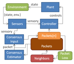
The whole control structure is called from updateBotComputations. Information about neighbors flows to and from the consensus estimator via the packet model.

Blue boxes

The blue boxes from the flowchart to the right represent functions that are defined in their own files. They are the building blocks of the consensus-based swarm model.

Plant

The interface between the agent and the environment. For the formation control implementation, this models an e-puck following a velocity vector.

Sensors

Consolidates information from the environment into a form readable by Consensus Input and the Controller.

Consensus Estimator

A discrete-time PI estimator that uses packet structs for its input and output.

Consensus Input

Injects the agent's own information into the estimator-communication cycle. In the formation control implementation, this step causes the estimates to follow the agents instead of converging to the starting location.

Controller

Uses the agent's sensory and consensus information to select a set of controls, sent to the plant.

Collision avoidance

The velocity output from the Controller is put through a collision avoidance algorithm. It is not shown in the flowchart because the algorithm has access to the positions of all the agents (information not known to any single agent).

Note: the present algorithm does not work very well.

Environment

The environment is a set of abstractions that encapsulate the control structure, simulating passage of time, motion of the agents, and lossy wireless communication.

Time model

The simulation advances in timesteps; equally spaced spans of time. Timesteps are the unit used in specifying the distance between discrete events, such as updating robot calculations or rendering. Their size (relative to other time-based units) is defined by the constant dT.

The main loop runs once per timestep. It updates the plant every timestep and makes calls to time-dependent update functions as needed.

Data model

Since all state data in the simulation can be associated with a robot, the only stored variable is a vector of N robots called bots. Each bot is individually represented as a struct, with the following fields:

• bots vector of N robots
  • state information the agent knows about itself
    • p position
    • angle rotational orientation
  • packets vector of N received packets (packet i of bot i is that agent's own estimate and always has an age of 0.)
    • age timesteps since received
    • v PI decision variable
    • w PI estimator state
  • u velocity chosen by Controller
  • lastUpdate timestep of last update
  • waitTime timesteps between last update and next update

Packet model

Consensus information is transferred between the e-pucks using wireless communications. The simulator transfers packets between robots on an asynchronous basis and includes the possibility of packet loss as a function of distance. Each robot's packets vector contains the most recently received packet from each of its neighbors. A robot will transmit its own consensus information just before its control structure is executed.

Packet loss is modeled by a cumulative Rice function, as advised by problem of Wi-Fi radio-fading simulation: Solution and applications. As distance between agents increases, the probability of receiving a packet decreases.

Visualizing packet loss

Packet loss can be easily visualized by setting the constant DRAW_CONNECTIONS to true.

Between two agents...

• a black line means at least one agent has a fresh packet from the other.
• a red line means neither has fresh data, but at least one is using stale data.
• no line means neither agent is using data from the other because the last communicated packet is older than PACKET_AGE_LIMIT.

Recording a movie

To record a run of the simulation, set MOVIE_FRAME_COUNT to the desired movie length, in frames. The movie will be saved as "movie.avi" in the same directory as the simulator M-file.

Movies are recorded as uncompressed AVIs because MATLAB does a poor job of compression. See Swarm Robot Project Documentation#Making Videos with Overlays.