Variable Frequency Electrosense

Introduction

Our objective was to build upon existing research being done at Northwestern utilizing Electrosense technology by testing if information can be derived from varying the emitter frequency. We sought to send sinusoidal waves at discrete frequencies between 100 Hz and 10 kHz and to read in the sensed wave using a PIC 32’s ADC. We then sent the gathered information to a PC for plotting and analysis. By mounting the sensor on a one dimensional linear actuator we are able to gather additional data about objects and perform object detection and identification algorithms. While our initial results have revealed exciting trends, farther research is necessary before any significant conclusions can be made. A video of the project is available on YouTube.

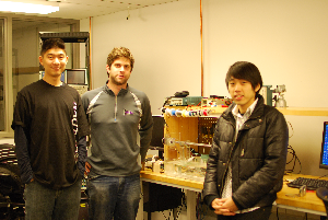
Team

• Tod Reynolds, EECS 2010
• Pill Gun Park, EECS 2011
• Joshua Peng, BME 2017

Assembly

sensor hookup

stepper motor hookup

limit switch hookup

Sensor Board hookup

Main Components

• Tank with Actuator/Sensor
• Circuitry with PIC32
• PC with processing interface

Steps to setting up

• Fill the tank with tap water until the level is just above the sensing board. Confirm that there are no leaks with the tank.
• Hook up the sensors and actuators to the circuitry.
  • The sensor ataches via a grey ribbon cable. The strip should be to the right and facing up on the board.
  • The stepper motor attaches by plugging in the 8 pin socket on the left hand, bottom side of the breadboard. The black and white wires should be at the top, and should be plugged into the same row on the board as the wires that run to the +12volt supply
  • The limit switches also attach by plugging in an 8 pin socket. This time orientation is not important, but one side of the switch must run to a resistor while the other attaches to ground and the signal out cable(yellow)
• Build & power the circuitry
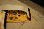
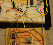
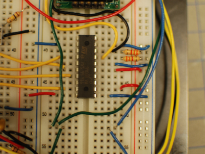
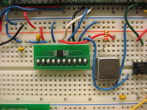
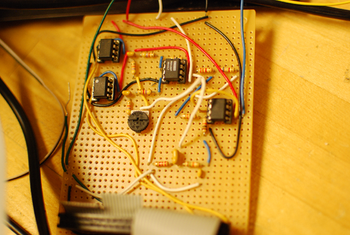
  • The sensor circuit is built on a solder board to ensure good conections between components. This board is attached to the solderless breadboard via 5 wires
  • Wire Color Code
    • Red: +5 volt supply. Plugs into same row as read wire running from supply on left hand side of board
    • White: ground, plugs into main ground rail on board
    • Black: -5 volt supply. Plugs into output of -5 volt regulator chip.
    • Green: sensor input. Plugs into row on breadboard that contains output from AD9833 amp as well as input to PIC
    • Blue: sensor output: plugs into blue wire on breadboard that runs into PIC
  • Power to the motor is from the 12volt regulator chip located at the top, left hand side of the breadboard
  • Power to the PIC is from the USB cable
• Hook up PIC to PC
  • USB cable for power
  • RS232 cable for communication (ensure that the proper drivers are installed)

Mechanical Design

Electrosense Water Tank

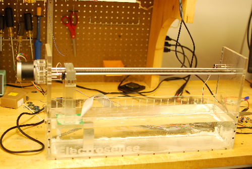
The tank is two feet long by 6 inches wide. It is made of laser cut acrylic and has the actuator built into it's side walls.

Linear Actuator

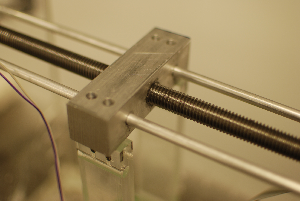
The linear actuator works by twisting a threaded rod. A machined bar with matching threads that the sensor is attached to will move because it is constrained from rotation. This actuator allows precise positioning but is very slow.

Electrical Design

Stepper Motor Circuit

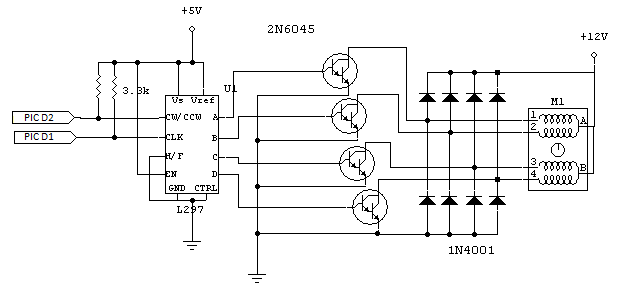
To drive the linear actuator a unipolar stepper motor is used. The stepper motor circuit takes in two signals from the PIC(Direction & Clock) and rotates the rod a corresponding number of steps.

stepper motor circuit

Parts

• IC's
  • 1x L297
  • 4x 2N6045
• Resistors
  • 3x 3.3K
• Diodes
  • 8x 1N4001

Signal Generation Circuit

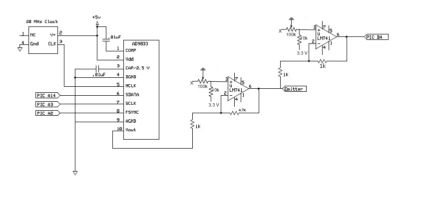
The AD9833 is a surface mount function generating chip that allows us to emit analog signals at discrete frequencies under control from the PIC. Because the the signal out of the chip is about 680mVpp an amplifier is used to boost the signal by a factor of 3.5. Also, because the signal out of the chip has the offset at about 0, differential amplifier has to be use to make 0 offset. After all, the signal out is about 2.4Vpp with 0 offset sinusoid wave.

AD9833 Circuit

Parts

• IC's
  • 1x AD9833
    • Surface Mount Chip
    • Custom PCB
  • 1x Op amp(LM741)
• Capacitors
  • 2x.01uF
• Resistors
  • 1x 1K
  • 1x 4.7K
  • 1x 10k
  • 1x 100k potentiometer
• Miscellaneous
  • 20 MHz Clock

Signal Amplification/Level Shifting Circuit

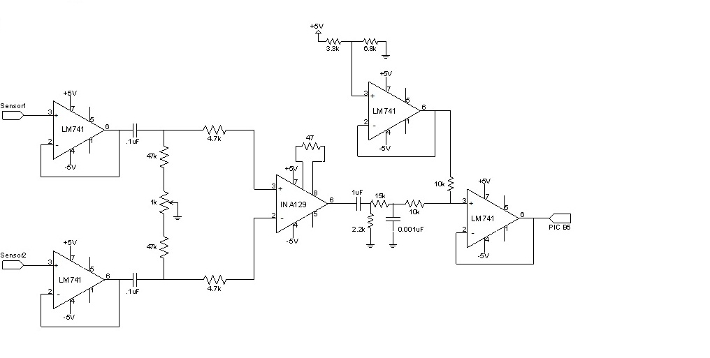
The sensed wave is generated by reading in the two waves at the sensor electrodes and comparing their signals.

• Each signal is initially buffered using a voltage follower
• Two signals are run though balancing circuitry to allow for a "zeroing" of the sensor

(make sure to adjust the balancing circuitry with potentiometer before the test)

• Two signals serve as inputs to Instrumentation amp which has a fixed gain of 1000
• Output signal is run through a bandpass filter
• Final signal is level shifted so that it can be read into the PIC's ADC which requires the signal be between 0 an 3.3 volts.

Note that this circuit is built in solder due to the extremely small voltage changes that need to be detected between the two sensed waves by the instrumentation amp.

signal amplification circuit

Parts

• IC's
  • 3x Op Amps(LM741)
  • 1x Inst Amp(INA129)
• Capacitors
  • 2x .1uF
  • 1x 1uF
  • 1x .001uF
• Resistors
  • 1x 1K Potentiometer
  • 2x 47K
  • 2x 4.7K
  • 1x 2.2K
  • 1x 15K
  • 2x 10K
  • 1x 6.8K
  • 1x 3.3K
• Miscellaneous
  • 50 Pin Header
  • Solder Board

Code

PIC Code

The PIC completes 5 main tasks:

• controls the AD9833 chip to generate voltage sinusoids
• receives the emitted and received waves and generates values corresponding to the analog signals such that each sinusoid period is 16 points long for each of the 19 frequencies
• calculates the FFT of the emitted and received waves
• controls the motor and linear actuator
• sends data to the PC (Processing) via RS232

Download the full version of PIC code

AD9833 Chip control

AD9833 is supposed to function under SPI control, however we found that bit-banging the registers was more reliable. The chip requires 16 binary bits for its input. The ad9833_set_freq(int value[]) function will send an array of binary numbers to the AD9833 chip. In this function, if the binary number is 0, we set the SDATA pin to low and if the binary number is 1, we set the SDATA pin to high. This process is performed for all 16 bits. According to the datasheet for AD9833, see here, the chip reads the data when FSYNC is low and at the low edge of the SCLK signal. Therefore, we set the FSYNC pin to low only when we are sending SDATA bits. Also, we initially set the SCLK pin to high and then set it back to low right after we send out SDATA.

#define PIN_A2			LATAbits.LATA2  //FSYNC
#define PIN_A3			LATAbits.LATA3	//SCLK
#define PIN_A14			LATAbits.LATA14	//SDATA

//send the AD9833 16 bits
void ad9833_set_freq(int value[]){
	 int i;
	 PIN_A3 = 1;                          // set SCLK pin high
	 PIN_A2 = 0;                          // set FSYNC pin low
	 for (i=0;i<=BITS16-1;i++){
	   PIN_A3 = 1;                        // set SCLK pin high
	   Delayms(1);
	     if (value[i] == 0){
	       PIN_A14 = 0;                   // set SDATA pin low
	     }
	     else {
	       PIN_A14 = 1;                   // set SDATA pin high
	     }
	   Delayms(1); 
	   PIN_A3 = 0;                        // set SCLK pin low
	   Delayms(1); 
	 }
	 PIN_A3 = 1;                          // set SCLK pin high
	 PIN_A2 = 1;                          // set FSYNC pin high
	 Delayms(3);
}

In order to generate a wave from an AD9833 chip, we need to reset the chip and send certain control bits to configure the type of wave that will be sent out. Then, we send the lsb and msb of the frequency register value. This value will be saved in the frequency register of the chip and will be used to calculate the actual frequency of the output wave. Next, we have to "un-reset" the chip. This function will generate sine waves if you give a msb and lsb as its parameter.

void generateWave(int msb[], int lsb[]){
        int ad_sine[BITS16] = {0,0,1,0,0,0,0,0,0,0,0,0,0,0,0,0}; // reset the chip and set output to be a sine wave
	int unreset[BITS16] = {0,0,0,0,0,0,0,0,0,0,0,0,0,0,0,0}; // unreset the ad9833 chip.
        ad9833_set_freq(ad_sine);
        ad9833_set_freq(lsb);
	ad9833_set_freq(msb);
	ad9833_set_freq(unreset);
}

The frequency of actual wave out of chip is calculated using the equation below and our master clock frequency, Fmclk is 20 MHz.

                   fout = (Fmclk/2^28) * frequency register value.

More details on the AD9833 chip can be found here.

Receiving Waves and Calculating Sampling Frequencies

We will read in two different sine waves from the analog inputs B4 and B5.

• B4: Emitted wave
• B5: Received wave

We are using T3 timer interrupt to sample the emitted wave and received wave. The sampling frequency of the timer is calculated to produce 16 points in one period of the sine wave. Therefore, we need 19 different sampling frequencies for all sine waves from 100Hz to 10KHz. With the PR value equation from Lab4, we set our global int variable 'samfreq' equal to the PR values we calculated for each sampling frequency.

 void initInterruptController(void)
{
	// init Timer3 mode and period (PR3) 
	OpenTimer3( T3_ON | T3_PS_1_1 | T3_SOURCE_INT, samfreq); 	
	mT3SetIntPriority( 7); 	// set Timer3 Interrupt Priority
	mT3ClearIntFlag(); 		// clear interrupt flag
	mT3IntEnable( 1);		// enable timer3 interrupts
}

Sampling Frequency and PR value for each input frequency are provided in table below.

Input Frequency	Sampling Frequency	PR Value(samfreq)
100	1600	0xC34F
200	3200	0x61A7
300	4800	0x411A
400	6400	0x30D3
500	8000	0x270F
600	9600	0x208D
700	11200	0x1BE6
800	12800	0x1869
900	14400	0x15B3
1000	16000	0x1387
2000	32000	0x09C3
3000	48000	0x0682
4000	64000	0x04E1
5000	80000	0x03E7
6000	96000	0x0341
7000	112000	0x02CA
8000	128000	0x0270
9000	144000	0x022B
10000	160000	0x01F3

FFT

A good FFT reference and explanation is found here.

/** Interrupt Handlers *****************************************/
// timer 3 interrupt
void __ISR( _TIMER_3_VECTOR, ipl7) T3Interrupt( void)
{
	int i;
	
        sampleBuffer1[sampleIndex].re = ReadADC10(0); // read the ADC from B4 into the real part
	sampleBuffer1[sampleIndex].im = ReadADC10(0); // read the ADC from B4 into the imaginary part

	sampleBuffer2[sampleIndex].re = ReadADC10(1); // read the ADC from B5 into the real part
	sampleBuffer2[sampleIndex].im = ReadADC10(1); // read the ADC from B5 into the imaginary part
	
	// you could shave a little time off this ISR by just zeroing the .im value once, outside the ISR

	// increment the sampleIndex
	if (sampleIndex == (N-1))
	{
		sampleIndex = 0;
	}
	else
	{
		sampleIndex++;
	}	 

	// clear interrupt flag and exit
	mT3ClearIntFlag();
} // T3 Interrupt

void computeFFT()
{
	// when using 256 samples, we measured this function to take about 500 microseconds
	// (not including the time to send rs232 data)
	int i;
	
	// generate frequency vector
	// this is the x-axis of your single sided fft
	for (i=0; i<N/2; i++)
	{
		freqVector[i] = i*(SAMPLEFREQ/2)/((N/2) - 1);
	}
	mT3IntEnable(0); //turns off interrupt while computing FFT
	
	for (i=0; i<N; i++)
	{
		if (i<sampleIndex)
		{
			// old chunk
			calcBuffer1[i+(N-sampleIndex)] = sampleBuffer1[i];
			calcBuffer2[i+(N-sampleIndex)] = sampleBuffer2[i];
		}	
		else // i >= sampleIndex
		{
			// new chunk
			calcBuffer1[i-sampleIndex] = sampleBuffer1[i];
			calcBuffer2[i-sampleIndex] = sampleBuffer2[i];
		}	
		
	}	

	// load complex input data into din
	mips_fft16(dout1, calcBuffer1, fftc, scratch1, log2N);
	mips_fft16(dout2, calcBuffer2, fftc, scratch2, log2N);	

	// compute single sided fft
	
	for(i = 0; i < N/2; i++)
	{
		singleSidedFFT1[i] = 2 * ((dout1[i].re*dout1[i].re) + (dout1[i].im*dout1[i].im));
		phase1[i] = atan2(dout1[i].im,dout1[i].re);
		singleSidedFFT2[i] = 2 * ((dout2[i].re*dout2[i].re) + (dout2[i].im*dout2[i].im));
		phase2[i] = atan2(dout2[i].im,dout2[i].re);
	}
	
	computeFFTflag = FALSE;

	// do something with dout
	mT3IntEnable(1); //turn interrupt back on
}

Motor Control

The Stepper motor circuit requires two inputs:

• Direction pin- D2 on the PIC
• Clock Signal- D1 on the PIC

We are using the interrupt handler for communication with Processing. The interrupt first checks which type of interrupt flag was generated (receive or transmit). If the interrupt was a "receive" interrupt, it first reads the key pressed and echos it back to the terminal. It then goes into a switch statement depending on the letter. The letters are described below:

• 'm' - make the motor move
• 'd' - take data at every half inch motor move
• 't' - stop motor movement
• 'f' - motor moves forward until stop requested
• 'r' - motor moves in reverse until stop requested
• 'a' - accelerates the motor
• 'l' - slows down the motor
• 'x' - while motor is stopped, sends data to Processing for further calculation and plotting
• 'c' - sends the motor to the zero position

// UART 2 interrupt handler
// it is set at priority level 2
void __ISR(_UART2_VECTOR, ipl2) IntUart2Handler(void)
{
	char data;
	// Is this an RX interrupt?
	if(mU2RXGetIntFlag())
	{
		// Clear the RX interrupt Flag
		mU2RXClearIntFlag();
	
		data = ReadUART2();
		// Echo what we just received.
		putcUART2(data);
		
		
		switch(data)

		{	
			case 'm':	//move
					move = TRUE;
				break;
			case 'd': 	//take data while moving
					data = TRUE;
				break;
			case 't':	//stop
					move = FALSE;
					data = FALSE;
				break;
			case 'f':	//forward
					DIR = Forward;
				break;
			case 'r':	//reverse
					DIR = Reverse;
				break;
			case 'l':	//slow
					speed++;
				break;
			case 'a':	//accel
					speed--;
				break;
			case 'c':	//calibrate
					calibrate = 1;
				break;
			case 'x': // get data
					cf++;
					wave(cf);
					Delayms(1000);
					computeFFT();
					//Delayms(500);
					sendDataRS232();
					if (cf == 19){
						cf = 0;
						notmove = 0;
						//move == TRUE;
					}
				break;	
		}			

		// Toggle LED to indicate UART activity
		mLED_0_Toggle();
 
	}

	// We don't care about TX interrupt
	if ( mU2TXGetIntFlag() )
	{
		mU2TXClearIntFlag();
	}
}

The code below is the infinite while loop in the main() function of our code. In order to move the sensor a half inch, our stepper motor will proceed through 1288 steps. After 1288 steps, the motor will stop moving and it will start to read in and send data. After it sends data to Processing, the motor will start to move again. If the stepper motor clock pulse periods are decreased, the motor will move faster. We control the motor speed with Delayms(speed). If 'speed' ('speed' is an integer variable) is incremented, then the motor slows down and if 'speed' decremented, then the motor will accelerate.

		while(1) //2575 steps = 1 inch
	{	
		if (calibrate == 1){    //calibrate button from process pressed
			dcalibrate();
			calibrate = 0;
		}
		while (move == TRUE){
			CLK = 0;
			Delayms(speed);
			CLK = 1;	
			Delayms(speed);
			step2++;
			
			if(INPUT_A9 == FALSE){
				step = 0;
				DIR = 1;
					while(step<200) {
					CLK=0;
					Delayms(speed);
					CLK=1;
					Delayms(speed);
					step++;
					}
			}
			if(INPUT_A10 == FALSE){
				step = 0;
				DIR = 0;
					while(step<200) {
					CLK=0;
					Delayms(speed);
					CLK=1;
					Delayms(speed);
					step++;
					}
			}
			if(step2 >= 1288){
				step2 = 0;
				//move = FALSE;
				if(data == TRUE){
				    cf++;
				    wave(cf);
				    Delayms(1000);
				    computeFFT();
				    sendDataRS232();
				    notmove == 1;
				    while(notmove == 1){
				    }
			      }
			}
			
		}

	}
CloseOC1();
} //end main

//sends the motor to initial position
void dcalibrate(){
	DIR = Reverse;
	while(INPUT_A10 == TRUE){
		CLK = 0;
		Delayms(speed);
		CLK = 1;	
		Delayms(speed);
	}
		step = 0;
		DIR = Forward;
		while(step<200) {
			CLK=0;
			Delayms(speed);
			CLK=1;
			Delayms(speed);
			step++;
		}
} 

Sending Data to the PC (Processing)

We send 7 variables out to the PC (Processing) via RS232. We send out the frequency array (256 points and 256 zeros) that holds the frequency values used in the FFT, the magnitude portion of the FFT of the emitted wave, the magnitude portion of the FFT of the received wave, the phase portion of the FFT of the emitted wave, the phase portion of the FFT of the received wave, the voltage sine wave values for the emitted wave, and the voltage sine wave values for the received wave.

vvoid sendDataRS232()
{
	int i;
	char RS232_Out_Buffer[128]; // max characters per line (line feed and carriage return count)
	
	sprintf(RS232_Out_Buffer,"\n\rSTART\n\r"); //print START. MATLAB uses this as a start delimiter
	putsUART2(RS232_Out_Buffer);
	
	sprintf(RS232_Out_Buffer,"ROWS=%d\n\r", N); //print the number of rows, so matlab can make the correct sized buffer
	putsUART2(RS232_Out_Buffer);
	
	for(i = 0; i < N; i++)
	{
		sprintf(RS232_Out_Buffer,"%d %d %d %f %f %d %d\n\r",freqVector[i], singleSidedFFT1[i], singleSidedFFT2[i], phase1[i], phase2[i], calcBuffer1[i].re, calcBuffer2[i].re);
		putsUART2(RS232_Out_Buffer);
	}
	
	sprintf(RS232_Out_Buffer,"END\n\r"); //output end so matlab knows we're done
	putsUART2(RS232_Out_Buffer);
	
}
  

• Full version of PIC code

Processing

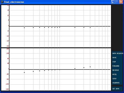
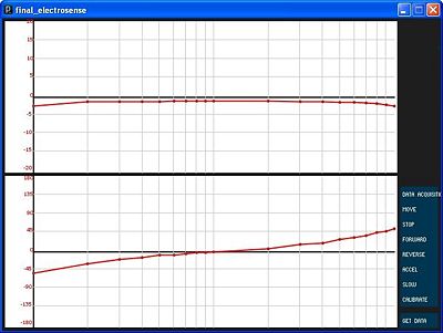
The Processing code will display a window on the computer monitor that allows the user to control the motion of the linear actuator and emitter/sensor board, run through a single routine of calculation and plotting, and run through full object identification and object detection routines.

The screenshot on the left is when it is currently calculating and plotting. The screenshot on the right is after it has finished calculating and plotting.

Buttons

Sensing Control

• Calibrate: returns the emitter/sensor board to the zero position. Unless it is in the middle of calculating and plotting, the board will immediately head in the reverse direction until it hits the limit switch and then it will go forward 200 steps so that the limit switch is completely released. All of our tests have been designed and analyzed according to and starting from this zero position. Once the Calibrate button is pushed, this process cannot be stopped unless someone flips the PIC power switch or the +12V/-12V power switch, etc.
• Move: activates the linear actuator so that the board can move
• Get data: activates calculation and plotting (runs the Object Detection routine)
• Data acquisition: activates calculation and plotting when the motor stops at every half inch

Linear Actuator Control

Note: for these buttons to have any effect, the "Activate" button needs to be pressed before these buttons

• Stop: board will stop moving (if it was already moving)
• Forward: board will move forward (if not already moving forward) at a constant speed
• Reverse: board will move reverse (if not already moving reverse) at a constant speed
• Accelerate: board will increase speed (by decreasing the delay between clock pulses of the bipolar stepper motor by 1 ms)
• Slow: board will decrease speed (by increasing the delay between clock pulses of the bipolar stepper motor by 1 ms)

Object Detection

• In order to run the Object Detection routine, you must press the "Data Acquisition" and "Move" in sequence.
• The board will move a halfinch forward from its current position, perform calculations and plotting after it stops, and then it will repeat this process until it hits the limit switch at the end. In this case, the step and location (according to the hashes) in the text file output will be off by 1 index.

Object Identification

• The Object Identification routine is performed automatically when "Data Acquisition" and "Activate" are pressed in sequence.
• Once the board has stopped moving and all 19 magnitude and phase bode plot points have been calculated and plotted, the program will compare the bode plot with library of bode plots of different object type in which the object was directly underneath the sensor and display the object index of the object with the closest matching bode plot for magnitude and phase in the space between the buttons.
• Thus, the program will try to identify whatever is underneath the sensor at its current position after each calculation and plotting routine (each time it has moved and stopped).

Window Contents

• Magnitude and Phase Bode plots - an experimental magnitude and phase bode plot is plotted at 19 frequencies between 100Hz and 10kHz

• Display of Object Type and Object Location - assuming that the sensor passes an object as it moves forward and runs through routines, program will run through an algorithm to determine where the object is according to the hashes on the back and what the object type is according to a bode plot library

• Space for data display and debugging - You can uncomment some portions of our code to display the values of arrays and variables on the empty right side of the window. Currently, for a few seconds after a calculation and plotting routine (until the board finishes moving a halfinch), the program will display the 19 magnitude and phase points of the bode plot. It also currently continuously displays many of the variables used in the calc() function.

Code

Description of Functions

Our full Processing code is much too long to post here, so we will instead post a link below and at the end of this section to a zip file with the actual code with comments. Some important portions of code are posted underneath their descriptions. Please note that you need to install the "ControlP5" custom GUI element library for Processing 1.0 by Andreas Schlegel in order for this Processing program to work. The following section will describe what each function in our code does.

Download a zip file of our Processing code and the ControlP5 library.

initserial()

Processing is set up so that it is continuously looking for data on the rs232 lines and once it sees data it will automatically start retrieving it. Once the sensor has finished moving and fully stopped, the pic will send 7 arrays each with 512 data points to Processing. The first set of arrays (data points) retrieved are of the 100 Hz voltage sinusoidal signals emitted and sensed. Next, there is a delay in the PIC, the sampling frequency is adjusted, the frequency of the signals is increased to 200 Hz, the fft of the signals is calculated, and then the next set of arrays corresponding to the 200 Hz wave is sent out and received by Processing. This process is repeated until it goes through all 19 frequencies (100 Hz, 200 Hz, 300 Hz,…,10 kHz).

• vector of frequencies (x axis) used to calculate the fft in the PIC, note that the first half (first 256 points) is nonzero, the second half is deleted (all zeros) in the PIC because it is essentially the same as the first half but in reverse order (256 frequency points + 256 zeros)

• The magnitude portion of the FFT(calculated from PIC) of both emitted and sensed signals. (512 wave points each)

• The phase portion of FFT(calculated from PIC) of both emitted and sensed signals. First 256 points are of the emitted signal, second 256 points are of the sensed signal. (256 emitted wave points + 256 sensed wave points)

• y axis points of the emitted sinusoidal signal (512 emitted wave points)

• y axis points of the sensed sinusoidal signal (512 sensed wave points)

    // grab the data
   if ((line_received.length == 7) && (portNumber==0)){
      freq[index] = line_received[0];
      fft1[index] = line_received[1];
      fft2[index] = line_received[2];
      phase1[index] = line_received[3];
      phase2[index] = line_received[4];  
      sin1[index] = line_received[5];
      sin2[index] = line_received[6];
      index++; 

• Note that we use this “newdata” Boolean variable to ensure that once we start collecting data points, we will finish collecting all 512 data points before we can use the data points for calculating and plotting in the other functions.

important global variables and setup()

Some important variables:

• int k = 0;

frequency counter, k is incremented by 1 each time draw() is run. Once it reaches 19 (frequency of signals at 10 kHz), it set to 0 (frequency of signals at 100 Hz) again.

• int L = 512;

total number of data points retrieved from PIC each time data is sent over.

• float bx = width/3; | float by = height/3;

all the buttons and plots are laid out in the window using these 2 variables

The setup() function basically creates rectangles in which plot curves appear, initializes the font used, sets the frame rate, initializes the output text write, and initializes the controlP5 buttons.

draw()

The sequence in which our functions are carried out is important.

• “newdata” allows us to run the rest of the functions only if we have finished getting all the data from the pic via rs232 and we have not reached the final 19th frequency

• While it collecting data for each frequency, it records and plots the magnitude and phase bode plot points

• it creates or appends data to a text file ("bodeplotdata.txt") in the folder where this sketch is located.

• Once we reach the last frequency (k reaches 19), all the 19 points plotted in the bode plot will be connected with red curved line.

void draw() {
    if (newdata == true && k < 19) { 
     calc();
     output.println("afreq: "+afreq+" | bfreq: "+bfreq+" | mag1: "+mag1+" | mag2: "+mag2+ " | aphase: " +aphase+ " | bphase: " +bphase+ " | magratiolog: "+magratiolog+" |phasechange: "+phasechange+"|sinmaglog: "+sinmaglog); 
     //output.println(" ");
     output.flush();
     //output.close();
    if (k == 0){
     initiallize(); 
    }
    text("hi",50+5*k,100);
    strokeWeight(5);
    stroke(100);
    point(mappedfreq,mappedphase);
    point(mappedfreq,mappedsinmag);
    magbodedata[k] = mappedmag;
    phasebodedata[k] = mappedphase;
    freqbodedata[k] = mappedfreq;
    sinmagbodedata[k] = mappedsinmag;
    sumphase = sumphase + phasechange;
    sumsinmag = sumsinmag + sinmaglog;
    if (k<18){
    myPorts[0].write(getdata);
    } else {
      avgphase = sumphase/19;
      avgmag = sumsinmag/19;
      sumphase = 0;
      sumsinmag = 0;
      
      if (abs(avgphase)<20){
        text("Object detected:",int(width-buttonwidth-5),50);
        text("Steel Ball",int(width-buttonwidth-5),70);
       }  
      strokeWeight(2);
      stroke(255,0,0);
      beginShape(LINES);
      for (int i = 0; i<18; i++){
       vertex(freqbodedata[i],phasebodedata[i]); 
       vertex(freqbodedata[i+1],phasebodedata[i+1]);
      }
      endShape();
      beginShape(LINES);
      for (int i = 0; i<18; i++){
       vertex(freqbodedata[i],sinmagbodedata[i]); 
       vertex(freqbodedata[i+1],sinmagbodedata[i+1]);
      }
      endShape();
    }
    k++;
    newdata = false;
    
    if (k > 18){
      k = 0;
    }
  }
}

calc()

• The index of the peak points of the fft magnitude arrays of the emitted and sensed waves are found.

• The corresponding phase value when magnitude of the FFT hits the peak points is found.

• Calculate 20*log(mag2/mag1). mag2 is peak points of the fft magnitude arrays of the received wave and mag1 for emmited wave.

• Calculate the phase difference between two signal.

 void calc(){
  for (int i=0;i<L-5;i++) {
    sfft1[i] = fft1[i+5];
    sfft2[i] = fft2[i+5];
  }
  mag1 = max(sfft1);
  mag2 = max(sfft2);
  for (int i=5;i<L;i++) {
	if (fft1[i] == mag1) {
		a = i;
	}	
	if (fft2[i] == mag2) {
		b = i;
	}
  }
  afreq = freq[a];
  bfreq = freq[b];
  aphase = phase1[a];
  bphase = phase2[b]-PI;
  
  magratio = mag2/mag1;
  
  phasechange = ((bphase - aphase)/(2*PI))*360;
  if (phasechange > 180){
   phasechange = phasechange - 360; 
  } else if (phasechange < -180){                                                                                  
   phasechange = phasechange+360; 
  }
  
  msin1 = max(sin1)-min(sin1);
  msin2 = max(sin2)-min(sin2);
  sinmagratio = msin2/msin1;
  sinmaglog = 20*log(sinmagratio)/log(10);
   
  afreqlog = log(afreq)/log(10);
  bfreqlog = log(bfreq);  
  magratiolog = 20*log(magratio)/log(10);
    
  mappedsinmag = map(sinmaglog,-20,20,gwh+5,5);
  mappedmag = map(magratiolog,-80,80,2*gwh+15,gwh+10);
  mappedphase = map(phasechange,-180,180,gwh+10,height-5);
  mappedfreq = map(afreqlog,2,4,50,625);
}

initialize()

• Clears the bode plots

Download a zip file of our Processing code and the ControlP5 library.

Test Results and Analysis

In the limited time between getting our circuit to function correctly with the Processing program and demostrating our project, we were only able to run a number of trials scanning past different objects to determine object type and object location. Our test results seem to indicate some trends but we cannot make any firm conclusions because this is only a first pass of experiments, hopefully the results obtained thus far will warrant future research.

Experimental Dimensions

Water tank measurements:

Emitter/sensor board = square with equal length and width = 3.19in / 81.02mm

Distance from floor to emitter/sensor board = 3.13in / 79.50mm

Distance from center of board to side of water tank = 3.13in / 79.50mm

Bipolar stepper motor measurements:

1 inch (25.4mm): 2576 steps

full distance of water tank the board can traverse (limit switch to limit switch) = 18.5 inches (470mm)

full distance in steps = 47656 steps

37 full halfinches in 18.5 inches (full distance)

1 halfinch (12.7mm) = 1288 steps

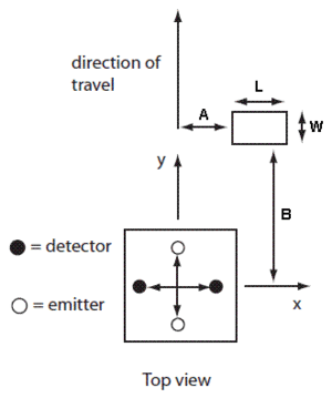
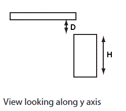
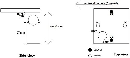
Geometry of test case

Test Cases and Results

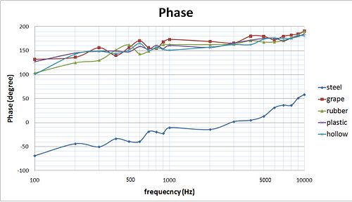
A sphere ball located between E1 and D1 as figure above. 5 different types of 1 inch sphere ball were used. (Steel, Rubber, Plastic, Hollow, and Grape)

you don't know the impedance properties of the environment, and you don't know exactly how your circuit is working. So let's get rid of the first one by creating an artificial environment of known properties.

Bode plots for different five objects and no object

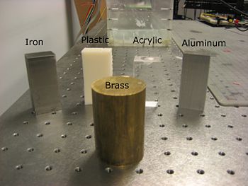
Aluminum

L = 1.25in / 31.69mm

W = 0.58in / 14.76mm

D = 0.36in / 9.15mm

H = 2.77in / 70.29mm

Iron

L = 1.26in / 31.88mm

W = 0.96in / 24.32mm

D = 0.39in / 9.84mm

H = 2.74in / 69.60mm

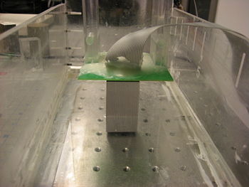
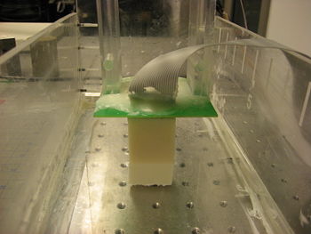
Acrylic (flipped so that the well is on the bottom facing the floor)

L = 1.26in / 32.00mm

W = 0.99in / 25.10mm

D = 0.80in / 20.54mm

H = 2.33in / 58.9mm

Plastic

L = 1.36in / 34.62mm

W = 0.76in / 19.24mm

D = 0.39in / 9.93mm

H = 2.74in / 69.51mm

Grape on acrylic block

One grape was put in the small well etched on the top face of the acrylic block.

Grapes were approximately 20mm diameter spheres.

D = 0.393in / 10mm

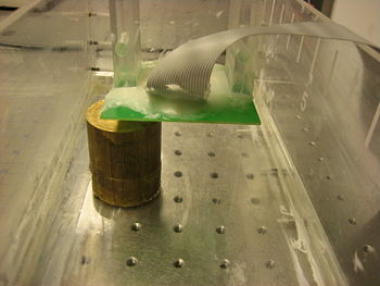
Brass cylinder

Diameter (L and W) = 1.75in / 44.61mm

D = 0.52in / 13.25mm

H = 2.61in / 66.19mm

Test Results

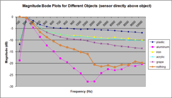
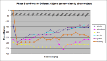
Bode plots for different objects with the emitter/detector board directly above the object.

Aluminum seems to have a characteristic response significantly different than the other objects.

For this experiment, all objects were placed in the water tank underneath the center of the board approximately at these specifications.

A = 0.00in / 0.00mm

B = 0.00in / 0.00mm

The recorded data and excel plots can be found here.

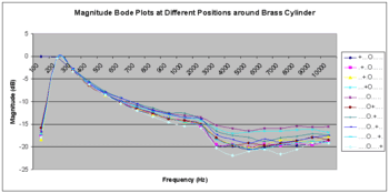
Bode plots as the board moves past a brass cylinder

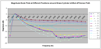
Especially at higher frequencies (4kHz to 10kHz), the magnitude values are the greatest when the board is directly above the brass cylinder.

For this experiment, the brass cylinder was placed in the water tank such that the center of the board would pass over the brass cylinder.

A = 0.00in / 0.00mm

B = 1.48in / 37.60mm

The recorded data and excel plots can be found here.

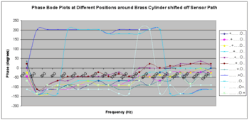
Bode plots as the board moves past a brass cylinder shifted off to the side

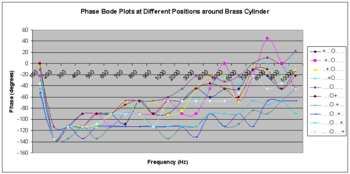
There is a big jump and plateau for several frequencies in the 3 phase bode plot curves where the board is near the object.

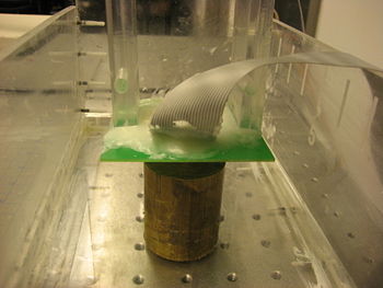
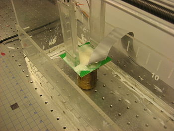
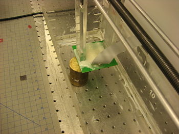
For this experiment, the brass cylinder was placed in the water tank shifted from the midline such that the detector electrodes on the underside of the board would pass over the brass cylinder.

A = 0.80in / 20.00mm

B = 4.45in / 113.07mm

The recorded data and excel plots can be found here.