Design and Control of a Pantograph Robot
Overview
The goal of this project was to design and build a 2-DOF Pantograph Robot. The user would be able to specify and X and Y location for the end point of the pantograph, along with different paths that the robot arm could take. The basic circuit design and computer code was taken from the High Speed Motor Control project and adapted to work with our robot design and motors.
Kinematics
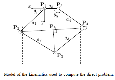
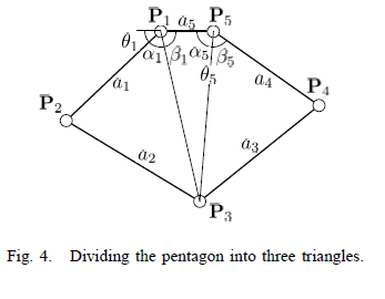
The kinematics for our robot design were derived from The Pantograph Mk. II - A Haptic Instrument. The forward and inverse kinematics as used in the MATLAB program are shown below, along with diagrams from the paper showing how the reference frames are defined in our setup. These angles are all calculated in radians, other parts of the programs convert this to degrees for graphing and user interfaces. The full programs can be found in the zip files below.
For our current robot arm, the distances a1, a2, a3, and a4 are all equal to 15 centimeters. The distance between the two motors, a5, is 2.75 inches which is equal to 6.985 centimeters.
There are a few differences in the notation on the diagrams and what is used in the code. Motor 1 in the robot is located at P1 on the diagram, and Motor 2 is at P5. The angle of Motor 1 in the diagram is shown as theta1, and the angle of Motor 2 is referred to as theta5. In the code, L1 corresponds to a1, L2 to a2, and so on. In the forward kinematics, the theta variable in the code corresponds to theta1, and alpha corresponds to theta5. In the reverse kinematics L13 is the distance from P1 to P3, and L53 is the distance from P5 to P3. Again, alphaOne corresponds to the angle of Motor 1, and alphaFive is the angle of Motor 2.
Forward Kinematics
x2 = L1 * cos(theta);
y2 = L1 * sin(theta);

y4 = L4 * sin(alpha);
x4 = L4 * cos(alpha) - L5;

two_to_four = sqrt((x2-x4).^2 + (y2-y4).^2);

two_to_h = (L2^2 - L3^2 + two_to_four.^2) ./ (2 * two_to_four);

yh = y2 + (two_to_h./two_to_four).*(y4-y2);
xh = x2 + (two_to_h./two_to_four).*(x4-x2);

three_to_h = sqrt(L2^2 - two_to_h.^2);

x3 = xh + (three_to_h./two_to_four) .* (y4-y2);
y3 = yh - (three_to_h./two_to_four) .* (x4-x2);
Inverse Kinematics
L13 = sqrt(x3.^2+y3.^2);
L53 = sqrt((x3+L5).^2 + y3.^2);

alphaOne = acos((L1.^2 + L13.^2 - L2.^2)./(2.*L1.*L13));
betaOne = atan2(y3,-x3);
thetaOne = pi - alphaOne - betaOne;

alphaFive = atan2(y3,x3+L5);
betaFive = acos((L53.^2 + L4.^2 - L3.^2)./(2.*L53.*L4));
thetaFive = alphaFive + betaFive;
Mechanical Design
The mechanical design is essential in order for the user to be able to accurately control the pantograph robot. The most important factors in accurate control are friction and mechanical coupling between the motors and arms. We also made it out goal to minimize the vertical deflection at the end of the arms. In this section I will go over how the design aims to meet these goals, the issues I ran into and possible areas of improvement.
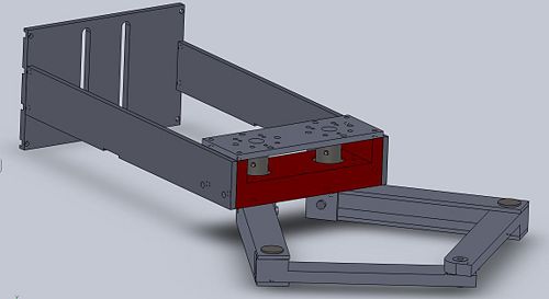
The entire CAD assembly of the pantograph robot can be seen at the right. We can see a mounting piece used to attach the robot to an 80/20 frame is attached to the rear of the robot on either side of the "shoulders" (pictured in red). These "shoulder" are the base of the entire design. A mounting plate for the attachment of various size motors is attached to the top, below which two couplings are set in counter-bores within the "shoulder". These couplings attach the motors to the left and right "biceps", the upper part of the arms. These "biceps" are then attached to "forearms", the lower part of the arms. The "forearms" are then attached to the "biceps" and to each other with specially made pins.
To keep the design lightweight all of the large components are made from 6061 Aluminum. Both the couplings and the pins were made from W1 Tool Steel on account of its strength and ease of machining. Their are two other special components that were custom made for this robot, not mentioned in the above paragraph, the bearings and shims located at the joints. The bearings were made from oil-filled bearing grade bronze and the shims were punched out of .005" Teflon sheet stock. The bearings were machined as opposed to being purchased for several reasons. The first reason is that size restrictions seriously limited the selection of ball or roller bearings available. Additionally, due to the speeds and forces imposed on the robot arm bearings with a lot of moving parts would add unnecessary complexity to the assembly.
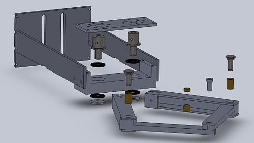
We initially believed that friction would be the largest hurdle to overcome, therefore the base of the design is focused on reducing friction. We chose to use 26mm Thrust Bearings to support the load of the arms at the "shoulder" as well as reduce friction. To the right we can see and exploded view of the entire assembly. From this image we can see the thrust bearings (pictured in black) are sandwiched between the couplings and "shoulder" and between a pair of washers and the "shoulder" on the underside of the assembly. The "biceps" are then attached to the "shoulder" with a screw running through the center of the washer and bottom thrust bearing and into the bottom of the coupling. By tightening this screw the thrust bearings are firmly pressed between coupling and "shoulder" and "bicep" and "shoulder". This sandwiching of thrust bearings theoretically eliminates friction at the "shoulder" as well as vertical deflection at the end of the "biceps".
Circuit Design
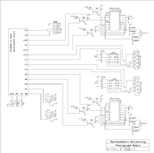
The complete circuit schematic for the current robot setup is displayed to the right. A brief description of the components in the circuit and what they do follows.
This is essentially one smaller circuit repeated for the second motor. Each motor is powered by an L298N H-bridge amplifier which is powered by 12 volts currently. These amplifiers are capable of sending out four different signals, however in this application the matching inputs and outputs are connected in parallel in order to increase the available current.
The PIC sends three signals to each H-bridge, one for each motor lead and an enable signal that activates the amplifier. These signals pass through 4N27 optoisolators to shield the motors from signal noise.
Each motor encoder is connected to an LS7083 encoder counter chip to allow the PIC to keep track of the motor angle in order to control the position of the end effector. This connection is made through a DB9 connector that interfaces with the plug attached to each motor.
There are two hall effect sensors that are mounted on the robot base and connected to the PIC. These allow the user to set the position of the arms by manually moving them at the beginning of the program until they are tripped by small magnets mounted on the robot arms.
The PC communicates with the PIC via RS232 using a MATLAB program. This allows the robot arm to be completely controlled by a PC once the program is loaded onto the PIC chip.
Parts List
| Electrical Components Needed. | Quantity | Data Sheets |
|---|---|---|
| PIC 32 on NU32 board | 1 | Introduction to the PIC32 |
| H-bridges L298 | 2 | data sheet |
| Optoisolators 4N27 | 6 | data sheet |
| Quadrature Up/Down decoders LS7083 | 2 | data sheet |
| Hall Effect Sensors | 2 | Hall Effect Sensor |
| 35V 9A Schottkey Diodes 90SQ035-ND | 8 | data sheet |
| Harmonic Drive RH-8D-3006 Actuator with 100:1 gear ratio and 1000 count per revolution encoder | 2 | data sheet |
| Power Supply | 1 | N/A |
MATLAB Code
The folder containing all of the code needed to control the robot in MATLAB is contained at File:Pantograph robot matlab.zip. An overview of how the program works is given below, and instructions for running the program are given in a later section.
Everything involving MATLAB with this robot is controlled from the me333gui, which is created by running the me33gui.m file. From this interface any button press or change of value is communicated with the PIC by calling a function that serves a specific purpose. Once the data has been processed, such as calculating an array of motor angles to create a specific path, this data is sent out to the PIC through serial communication. Comments contained in the beginning of each set of code explain exactly what that piece of code does.
Some things to note: The serial communication through MATLAB is fairly buggy right now and alternatives should be explored. One such alternative was recently brought to the group's attention, a method for using USB communication to communicate directly from a PC to a PIC without using serial. More information on that method can be found at this link: Building_a_PIC18F_USB_device.
Any changes to the physical setup, whether it be the lengths of the arms of the resolution of the motor encoder, need to be updated in the arm_constants.m file.
All data is currently sent to the PIC as int32 integers. These were originally int16 integers but the resolution of this specific encoder and gearhead mean that sometimes the desired encoder position will exceed the space available in a 16-bit integer.
The current limiting factor in data logging speeds is the rate at which the PIC sends data to MATLAB via RS-232. Because of the slow speed of this process it is not currently possible to update the graphs for every cycle of a looped path.
PIC Code
The folder containing the C code currently found on the PIC can be found at File:Pantograph robot PIC.zip.
The main piece of code that is constantly running is ArmControlMain.c. This controls constantly updating the encoder readings and calculating the error and resultant reference signals. The SerialFunctions.c file handles the processing of incoming serial data and outgoing data sent when a log is asked for. MotorCommands.c controls what happens when different motor functions are called. When editing these it is important to remember that the sign of these settings are crucial, a negative in the wrong place can cause the motor to spin in the wrong direction unexpectedly and potentially damage one of the arms.
Constants.c contains the important setup data that will need to be looked into at some point. This is all commented in the code, but it contains the predefined angular limits for the arms, along with predefined control gains, how frequently data is logged, how quickly to execute GO_TO commands and more.
Operating Instructions
The steps to operate the robot arm in its current configuration are as follows:
1. Plug in and check all connections. Connect the power USB cord for the PIC and the RS-232 cable to the laptop that will be running the MATLAB program. Plug in the multi-connector for the motors and encoders. Plug in the power supply leads to the vertical strip on the far right side to supply power to the motors. Plug in the hall sensor plugs in the marked space on the left side. The locations for each plug with description are as follows, for future reference:
- RS-232: Left side, rows 22-27 with the black wire at the row 22 position.
- Hall sensors: Motor 1 sensor rows 29-33, Motor 2 sensor rows 34-38. Motor 1 is the motor on the right side of the robot when standing behind it, where the coordinate system is defined from. The wires in each that are at row 29 and 34 respectively are marked with a black piece of electrical tape.
- 24V Motor Power Supply: Plug in connector anywhere along the vertical power/ground strip on the far right side. Make sure the black cable is lined up with the right side (ground).
- PIC power cable: Plugs into the USB connector on the PIC board.
- Multi-connector for motor leads and encoder cables: Plugs in on the right side of the circuit, bridging the small gap between the two right sections, from rows 35-44. The side of the connector that is full of cables goes on the left side of this gap.
2. Run the MATLAB program. Open MATLAB and run the me333gui.m file contained in the folder located in the MATLAB Code section of this page. This will open the GUI interface that sends commands to the robot arm. You may have to choose 'Add to path' if a window pops up telling you that the folder containing the M-file is not in the predefined path.
3. Connect to the COM port. There is a box in the GUI that says "COM#". Replace the # sign with the number of the serial port that the RS-232 cable is connected to and press connect. If you select an unavailable port an error message will appear in the main MATLAB command window. It will also list the available ports, the RS-232 cable should be one of those. If you accidentally choose the wrong port out of the available ones the MATLAB program will work but the motors will do nothing. Simply press disconnect and try a different port.
4. Home the arms. Turn on the PIC using the switch on the NU_32 development board. Before the robot can do anything the arms must be homed to determine what angle they are currently at. Move the arm attached to motor 2 by hand until it trips the hall sensor at approximately 180 degrees. LED 0 on the board will then turn off. Then move the other arm to roughly 0 degrees until the other hall sensor is triggered, which will turn off LED 1. The robot is now ready to run.
5. Choose a path and run it. There are currently three available options for controlling the robot arm. The 'Go To' option moves the end point of the arm to a user-defined position in the x-y plane. The duration of this move is set in the code on the PIC and can be easily adjusted, though not in the MATLAB interface. The 'Circle' option allows the user to define an ellipse by choosing the center point, radius in both X and Y directions, and length of time in seconds that the arm takes to trace it out. The 'Trace' option allows the user to define a path consisting of four points that the arm will trace out. In order to run any of these options, click on the radio button, type in your desired coordinates, and click Start.
6. Logging Data. In order to record and graph the encoder data, the motor must be running a Circle or Trace path, and the Loop Path option must be checked when the path command is sent. This tells the robot to repeat the circle or path until it receives another command. Once the arm has completed at least one cycle you can receive the data by pressing the Get Data button. Alternately, you can check the Continuous Update box which will continually ask the PIC for data and graph it. You can choose a graph of motor angles vs. time or x position vs. y position by choosing that selection before asking the PIC for data. Each graph displays the desired data and actual recorded data for each motor, allowing the users to see if any adjustments are needed in the gain values.
7. Adjusting the gains The robot arm is currently controlled by PID control based on the gains entered in the corresponding boxes in the GUI. The program will automatically send out these gains whenever a Circle or Trace command is sent, or you can press the Update button to send these new values to the PIC at any time.
Notes:
- In order to stop the arm in its current position the user can press Pause. A new path can then be chosen. Alternately, a new path can be sent while the PIC is running a different path and it should switch to the new path on the fly.
- If the arm stops suddenly it has most likely reach the predefined limits set in the PIC code to prevent the motors from damaging the arms. If this is the case the red warning LED on the breadboard will be lit. Simply move the arms by hand to a safe position and choose a different point or path.
- If you are experimenting with a low enough gain that the looped path it is following is not keeping up with the reference path, updating to a higher gain can cause sudden, violent movements due to the large error in the system. This should not damage the motors arms, however it is something to be aware of.
Usable Workspace
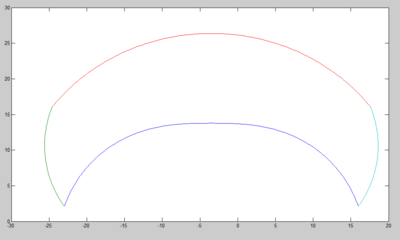
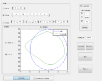
The usable workspace of the robot arm is limited by the predetermined angular limits on the arm which are defined in the constants.h file in the PIC code. The workspace of the robotic arm in its current configuration is shown in the image to the right. All units are the same as the ones used to define the arm constants, which in this case is centimeters, and the X and Y coordinates are the global coordinates used in the MATLAB GUI, where global zero is at the output shaft of Motor 1. In the current iteration, the limits were estimated through manual movement and checking of the arm clearances and are as follows:
| Measurement | Lower Limit | Upper Limit |
|---|---|---|
| Theta1 | -90 degrees (-25000 encoder counts) | 135 degrees (37500 encoder counts) |
| Theta2 | 45 degrees (12500 encoder counts) | 270 degrees (75000 encoder counts) |
| Theta2 - Theta1 | 40 degrees (11111 encoder counts) | 95 degrees (26388 encoder counts) |
At the moment the workspace is mostly limited by the maximum difference in angle between Theta1 and Theta2. This workspace can be seen in the image to the right. Although Theta2 is allowed to go to 270 degrees in theory, the furthest it ever goes is 230 degrees because it is not allowed to be more than 95 degrees greater than Theta1. This limit was set at 95 because at its most restrictive point that is the maximum angle the arms will allow, however in reality this physically possible angle increases as both arms move to either side. Moving the arms by hand it is obvious that Theta2 can actually reach 270 degrees, however our limits will not allow this. In the future perhaps a more complicated method of setting limits should be designed which takes this variation into account.
Known Bugs
- Occasionally the Get Data function will return an error. This is a recent phenomenon and the immediate cause is unknown. It appears that sometimes MATLAB does not completely convert the string data to integers, which prevents the program from calculating the angles. When the program attempts to multiply the DATA matrix by an integer, sometimes it returns an error that it cannot multiply a cell array by an integer. Simply press the Get Data button again and it should work properly. If the continuous update checkbox has been selected this error can cause the program to stop checking for updates. This has been observed in both Trace and Circle commands, for graphing both XY and Theta vs. time data. The error code is shown below.
??? Undefined function or method 'mtimes' for input arguments of type 'cell'.

Error in ==> arm_theta_plot at 25
theta1ref = DATA(:,1)*360/countsPerRev;

Error in ==> me333gui>getDataButton_Callback at 483
    arm_theta_plot(handles.axes3,DATA)

Error in ==> gui_mainfcn at 95
        feval(varargin{:});

Error in ==> me333gui at 52
    gui_mainfcn(gui_State, varargin{:});

Error in ==> @(hObject,eventdata)me333gui('getDataButton_Callback',hObject,eventdata,guidata(hObject))

??? Error while evaluating uicontrol Callback
- Sometimes when sending a path to the PIC, whether it is a Circle or Trace path, an error occurs in the serial communication and the command is not send. This is due to a timeout being reached during the write command, causing the program to hang. To solve this problem simply press the Start button again after the error message has appeared to reattempt sending the commands. The error code for this bug is as follows.
??? Error using ==> serial.fwrite at 184
A timeout occurred during the write operation.

Error in ==> arm_do_path at 39
fwrite(COM, [C_SET_PATH numPathPoints pathPICVector], 'int32');

Error in ==> me333gui>startButton_Callback at 403
        arm_do_path(COM, path)

Error in ==> gui_mainfcn at 95
        feval(varargin{:});

Error in ==> me333gui at 52
    gui_mainfcn(gui_State, varargin{:});

Error in ==> @(hObject,eventdata)me333gui('startButton_Callback',hObject,eventdata,guidata(hObject))
Preliminary Results
These are some of the results obtained from preliminary testing performed on June 11, 2010.
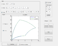
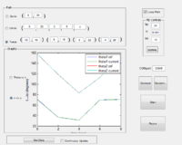
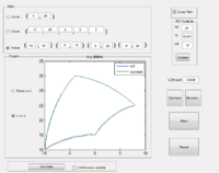
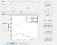
These first two graphs show the encoder data in both X vs. Y and theta vs. time for a trace pattern. The third graph shows the results when the arm was physically pushed on during part of the motion. Note that if too much force is applied to the arm it will cause slippage which will not show up in the encoder data.
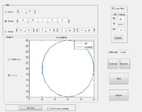
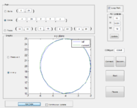
The next set of four graphs show encoder data when a circle path is defined. The first two show X vs. Y and theta vs. time data for a normal path, while the next two show the X vs. Y data for a path when the proportional gain is lowered. The values shown in the image are the values used for each path, and it is obvious how lowering the gain can affect the robot's ability to follow a defined path.
Next Steps
- Add a third degree of freedom: The original plan for this robot includes a third motor at the end point of the robot arm, allowing control of the angle of the end effector. This will require only slight modifications to the circuitry and coding. The angle from P2 and P3 in the kinematics can easily be determined which will allow the user to define the end effector angle by adding or subtracting from that angle. The GUI will need to be modified to accept an angle parameter, and the functions that it calls will need to send that extra parameter to the PIC. In the PIC code, the control functions for the first two motors will need to be replicated for the third.
- Use a more advanced encoder counter: Adding a third motor will require the use of different encoder counter chips, as the PIC32 has a limited number of clock pins available. The two current leading options are the LS7166 and the LS7366R. Preliminary testing indicates that the LS7366R is more robust, however update speeds are a concern as it is limited by the speed of SPI communication with the PIC.
- Implement velocity control: The jacobian of the kinematics needs to be determined in order to derive the dynamics of the system. Through this it will be possible to control not only the position of the end effector but also the velocity, which is one of the ultimate goals of this project.
- Using Copley amplifiers: Eventually the L298 H-bridges will be replaced by Copley amplifiers, which will allow the PIC to control the current to the motors through a PWM signal rather than the voltage. This will allow for more refined velocity control.
- Improve PC communication with PIC: As mentioned in a previous section, there are a few bugs in the system that occur when the serial communication with the PIC does not work properly. These could be eliminated if a more robust system was used, and data logging would also be more useful if a faster communication protocol was implemented.
