Control with TrackCam Vision Feedback and MATLAB

Stripping Down Windows

To make the new computer that runs the control system run as efficiently as possible, all extraneous functionalities were turned off. There is not anti-virus software, no firewall, no https for the internet, and so on. Only the bare minimum is left. Below is a list of the remaining functions and what they do. Another thing to do to make MATLAB run faster is to set it to go to the Task Manager, go to Processes, right-click on MATLAB.exe and set it to Realtime priority.

Explorer.exe

This is the user shell, which we see as the familiar taskbar, desktop, and other user interface features. This process isn't as vital to the running of Windows as you might expect, and can be stopped (and restarted) from Task Manager, usually with no negative side effects on other applications.

nvsvc32.exe

Part of the NVIDIA graphics card drivers (Detonator). It should be left running on any system using Nvidia graphics hardware to ensure proper function.

MATLAB.exe

MATLAB

svchost.exe

an integral part of Windows OS. It cannot be stopped or restarted manually. This process manages 32-bit DLLs and other services. At startup, Svchost.exe checks the services portion of the registry and constructs a list of services that it needs to load. Under normal conditions, multiple instances of Svchost.exe will be running simultaneously. Each Svchost.exe session can contain a grouping of services, so that many services can be run depending on how and where Svchost.exe is started. This allows for better control and debugging.

lsass.exe

the Local Security Authentication Server. It verifies the validity of user logons to your PC or server. Lsass generates the process responsible for authenticating users for the Winlogon service. This is performed by using authentication packages such as the default, Msgina.dll. If authentication is successful, Lsass generates the user's access token, which is used to launch the initial shell. Other processes that the user initiates then inherit this token.

services.exe

This is the Services Control Manager, which is responsible for running, ending, and interacting with system services. Use this program to start services, stop them, or change their default from automatic to manual startup.

winlogon.exe

runs in the background. Winlogon is a part of the Windows Login subsystem, and is necessary for user authorization and Windows XP activation checks.

csrss.exe

This is the user-mode portion of the Win32 subsystem; Win32.sys is the kernel-mode portion. Csrss stands for Client/Server Run-Time Subsystem, and is an essential subsystem that must be running at all times. Csrss is responsible for console windows, creating and/or deleting threads, and implementing some portions of the 16-bit virtual MS-DOS environment.

smss.exe

This is the session manager subsystem, which is responsible for starting the user session. This process is initiated by the main system thread and is responsible for various activities, including launching the Winlogon and Win32 (Csrss.exe) processes, and setting system variables. After it has launched these processes, it waits for either Winlogon or Csrss to end. If this happens normally, the system shuts down; if it happens unexpectedly, Smss.exe causes the system to stop responding (hang).

ctfmon.exe

When you run a Microsoft Office XP program, the file Ctfmon.exe (Ctfmon) runs in the background, even after you quit all Office programs. Ctfmon.exe monitors active windows and provides text input service support for speech recognition, handwriting recognition, keyboard translation, and other alternate user input forms.

rundll32.exe

This program is part of Windows, and is used to run program code in DLL files as if they were within the actual program.

RTHDCPL.EXE

a process belonging to the Realtek HD Audio Control Panel and is bundled alongside Realtek sound cards and audio hardware. This program is a non-essential process, but should not be terminated unless suspected to be causing problems.

ipoint.exe

a process installed alongside a Microsoft IntelliMouse and provides additional configuration options for these devices. "This program is a non-essential process, but should not be terminated unless suspected to be causing problems.

System

a process which shows up on the tasks on mainly Windows XP, Windows 2003 server and later version of Windows. This is a default system counter and cannot be removed.

Shared Memory

One of the methods explored to make the system run as quickly as possible was to have MATLAB and the camera running on separate cores of the computer, so both could run in parallel. This would require for them to communicate through shared memory. At the bottom of this page is a .cpp program that communicates through shared memory. We ultimately did not take this approach because Windows appears to be quick enough for now. Eventually, a real-time operating system such as Linux RTAI would be preferred, but for the time being, Windows suffices. I will therefore not explain further how the shared memory option works. However, if it is ever needed, everything to communicate through shared memory is in that file.

Test of Sample Rates

Overview

To see if using Windows instead of a real-time operating system would be a viable option, we had to test how fast the sampling rate could be set to without losing samples. We tried two methods: the first was to output data on one computer and collect it on the same computer, and the second was to output data on one computer and collect it on another computer.

Single Computer Tests

Pulses
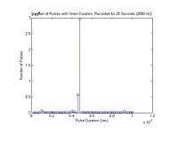
To run these tests, we used Measurement Computing Cards (mcc). Both were installed in the same computer. The MATLAB code that is at the end of this document was then run (testInputOutput.m). It creates an output wave that is a wave of alternating pulses. These were output at a predetermined rate. The input card kept on taking input all the time. Then, the duration of the input pulses was measured to see how long each pulse actually was as opposed to how long we wanted it to be. Plots of this were made, along with the standard deviation and the extra duration of each pulse. Using this method, we were able to see how fast we could feasibly run the alternate pulses without losing accuracy. Figure 1 shows that this test started to break down around 2000 Hz.

Figure 1: Number of pulses with given duration.

Two Computers

Pulses
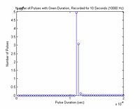
The next step was to output data on one computer and to input data on another. For output, we again used the mcc card. For input, however, we used a National Instruments (ni) card. Two programs were run for this test. The program run from the output computer was testOutput.m, and the one run on the input computer was testInputCard.m. With this simple modification to the setup, the test still ran fine at 10000 Hz, as can be seen in Figure 2.

Figure 2: Number of pulses with given duration.

Single Computer Again

Sine Wave
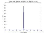
Following the tests with pulses, we decided to try to send a sine wave instead of a pulse, and to see at what output sample rate the frequency of the wave started to become inaccurate. This test is more practical, since in reality we would be sending sine waves and not pulses, and a little error in the output wave is acceptable in our applications. We used the same single computer setup as before, and ran the code inputOutputSineWave.m. A result of this test can be seen in Figure 3.

Figure 3: Frequency of sine wave with requested frequency of 50 Hz.

Sine Wave Sweep
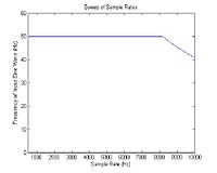
Finally, we decided to try a sweep of sine wave frequencies to determine exactly where the input frequency breaks down. The code that was run is called sweepOfSampleRatesSineWave.m. The results of this can be seen in Figure 4. This breakdown occurred at 8100 Hz.

Figure 4: Sweep of requested sample rates.

Integration of Systems

To begin

Make sure the National Instruments input and output cards are hooked up and set up with the new computer. On line 39 of the program “integrationTestPutSample.m”, make sure the right device number is chosen. As the program runs now, only the bottom two speakers are controlled, and the left and right speakers don’t move. Make sure the camera is calibrated properly. Run the .m file, and the ball should be bounced to an average height of 20 mm. This is a test of the closed feedback loop from the camera.

Contents of programs

The program consists of two separate programs. There is the MATLAB .m file, “integrationTestPutSample.m”, and the MEX-file, “skeleton.cpp”. The analysis of the data collected is done in MATLAB, where it can be seen in the beginning that a lot of matrices are set up to hold data. Then, the MATLAB program calls the MEX-file, which returns a lot of data, and that data is analyzed in MATLAB. The MEX-file itself takes the pictures and does image processing, calculating the centroid of each picture of the bouncing ball. All the functions in both the .m file and the .cpp file are documented within the programs.

Overview of operation of control system

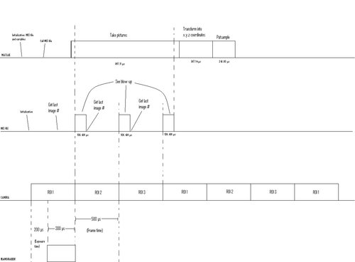
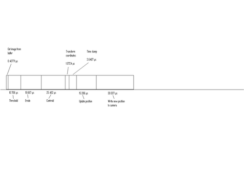
First, the camera and the framegrabber are initialized by allocating space in memory for the images that will be taken. Then, the camera starts taking pictures at a pre-specified rate (FRAME_TIME in the constants.h file). The three most recent pictures (real ball, reflected ball, and bar) are then taken from the image buffer and the coordinates of each centroid are calculated with some image processing algorithms. Then, these coordinates are used as input to another function in MATLAB to calculate x, y, and z coordinates for the ball and x and z coordinates for the bar. After that, the program checks if the ball is below 14.5 mm from the bar. If it is, half a period of sine wave is input into the speakers, and the ball is bounced back up. If the previous bounce of the ball was above 21 mm, the amplitude of the sine wave is reduced a little. If the previous bounce was below 19 mm, the amplitude of the sine wave is increased a little. This keeps the ball bouncing to approximately 20 mm. This loop then runs for as long as is specified, and afterwards the space allocated for the images is de-allocated.

Timing

The timing of the system is detailed on the timing diagrams (Fig 5 and 6). The idea, which is not fully implemented yet, is to have there be two pictures already taken when the MATLAB program calls the MEX-file, so that the program waits for only one more picture to be taken and then grabs all three and processes them all. To implement this, the frame time has to be just a little shorter than half of the total processing time, including the MEX-file processing and the MATLAB processing.

Figure 5: Sweep of requested sample rates.

Figure 6: Sweep of requested sample rates.

Code

Shared Memory

 
#include <windows.h>
#include <stdio.h>
#include <conio.h>
#include <tchar.h> 

#define BUF_SIZE 256
TCHAR szName[]=TEXT("Global\\MyFileMappingObject");
//TCHAR szMsg[]=TEXT("What's up (from the first process)?");
int szMsg;

int _tmain()
{
   HANDLE hMapFile;
   LPCTSTR pBuf;
   int ch,image;
   int coordinates[3];

   hMapFile = CreateFileMapping(
                 INVALID_HANDLE_VALUE,    // use paging file
                 NULL,                    // default security 
                 PAGE_READWRITE,          // read/write access
                 0,                       // max. object size 
                 BUF_SIZE,                // buffer size  
                 szName);                 // name of mapping object
 
   if (hMapFile == NULL) 
   { 
      _tprintf(TEXT("Could not create file mapping object (%d).\n"), 
             GetLastError());
      return 1;
   }
   pBuf = (LPTSTR) MapViewOfFile(hMapFile,   // handle to map object
                        FILE_MAP_ALL_ACCESS, // read/write permission
                        0,                   
                        0,                   
                        BUF_SIZE);           
 
   if (pBuf == NULL) 
   { 
      _tprintf(TEXT("Could not map view of file (%d).\n"), 
             GetLastError()); 

	  CloseHandle(hMapFile);

      return 1;
   }

   for (szMsg=0;szMsg<5;szMsg++) {
	   image = szMsg*2;
	   coordinates[0] = image * 2;
       coordinates[1] = image * 3;
       coordinates[2] = image * 4;

	   CopyMemory((PVOID)pBuf, coordinates, (3*sizeof(int)));

	   _cputs( "Type 'Y' to increment counter: " );
	   do
	   {
		  ch = _getch();
		  ch = toupper( ch );
	   } while( ch != 'Y' );

	   _putch( ch );
	   _putch( '\r' );    // Carriage return
	   _putch( '\n' );    // Line feed  
   }

   UnmapViewOfFile(pBuf);

   CloseHandle(hMapFile);

   return 0;
}

#include <windows.h>
#include <stdio.h>
#include <conio.h>
#include <tchar.h>
#pragma comment(lib, "user32.lib")

#define BUF_SIZE 256
TCHAR szName[]=TEXT("Global\\MyFileMappingObject");

int _tmain()
{
   HANDLE hMapFile;
   LPCTSTR pBuf;
   int i;
   double coordinates[3];
   int temp;
   const char *tempChar;

   hMapFile = OpenFileMapping(
                   FILE_MAP_ALL_ACCESS,   // read/write access
                   FALSE,                 // do not inherit the name
                   szName);               // name of mapping object 
 
   if (hMapFile == NULL) 
   { 
      _tprintf(TEXT("Could not open file mapping object (%d).\n"), 
             GetLastError());
      return 1;
   } 

   pBuf = (LPTSTR) MapViewOfFile(hMapFile, // handle to map object
               FILE_MAP_ALL_ACCESS,  // read/write permission
               0,                    
               0,                    
               BUF_SIZE);                   
 
   if (pBuf == NULL) 
   { 
      _tprintf(TEXT("Could not map view of file (%d).\n"), 
             GetLastError()); 

	  CloseHandle(hMapFile);

      return 1;
   }

   tempChar = (const char *) pBuf;
   temp = atoi(tempChar);
   do {
	for (i=0; i<3; i++){
		*(coordinates+i) = (double) (atoi((const char *) (&(*(pBuf+i)))));
	}
   } while (1);

   UnmapViewOfFile(pBuf);

   CloseHandle(hMapFile);
 
   return 0;
}

testInputOutput.m

clear all
close all
% set a desired sample rate of output
sampRate = 5000;
dt = 1/sampRate;
amp = 1;
% set input card's sample rate
sampRateIn = 50000;
% amount of time to acquire data
timeIn = 10;
trigger = timeIn*sampRateIn;

% creat input and output objects
AI = analoginput('mcc',0);
AO = analogoutput('mcc',1);

% add channels
addchannel(AI,[0:5],[1:6]);
addchannel(AO,[0:5],[1:6]);

% set up cards
set(AI,'SampleRate',sampRateIn)
set(AI,'SamplesPerTrigger',trigger)
set(AO,'SampleRate',ceil(1/500))

time = 1/sampRateIn:1/sampRateIn:timeIn;
t = 0:dt:timeIn;

% create an output wave that is just an alternating pulse
outputwave = zeros(length(t),1);
for jj = 1:floor(length(t)/2)
    outputwave(2*jj,1) = amp;
end
outputwave(:,2) = outputwave;
outputwave(:,[2 3 4 5 6]) = 0;

temp = rand(10);

% start acquisition
start(AI)
tic
a = 0;
% output data
for ii = 1:length(outputwave)
    while(toc<(dt*ii))
    end
    putsample(AO,outputwave(ii,:));
    %z = sampleMexFile(ii,ii,ii);
    %fft(outputwave);
    %fprintf('pause: %f\n',dt-time);
    %data(ii,:) = getsample(AI);
end

% collect data
data = getdata(AI);
stop(AI);
delete(AI)
clear AI

% get meaningful data from the channel that matters
meaningfulData = data(:,1);
plot(time,meaningfulData);

freqData = zeros(trigger,1);
counter = 0;
pulseCounter = 1;
% count number of pulses that have a specific duration
for ii = 2:trigger
    if (abs(meaningfulData(ii) - meaningfulData(ii-1)) < .05)
        counter = counter + 1;
    elseif ((counter ~= 0) && (ii-counter > 3))
        freqData(counter) = freqData(counter) + 1;
        pulseDuration(pulseCounter) = counter/sampRateIn;
        counter = 0;
        pulseCounter = pulseCounter + 1;
    elseif (ii-counter == 3)
        counter = 0;
    end
end

average = 1/sampRate;
figure
% create a graph of pulse durations
stem(time(1:2*average*sampRateIn),freqData(1:2*average*sampRateIn));
title(['Number of Pulses with Given Duration, Recorded for ',num2str(timeIn),' Seconds (',num2str(sampRate),' Hz)']);
xlabel('Pulse Duration (sec)');
ylabel('Number of Pulses');

averageDuration = 0;
for jj = 1:trigger
    if (freqData(jj) ~= 0)
        fprintf('%u pulses had duration of: %f \n',freqData(jj),jj/sampRateIn);
        averageDuration = averageDuration + (freqData(jj)*jj/sampRateIn);
    end
end
fprintf('\n');
averageDuration = averageDuration/sum(freqData);
fprintf('Average duration of pulses: %f \n\n',averageDuration);

standardDev = 0;
% find the standard deviation
for jj = 1:trigger
    if (freqData(jj) ~= 0)
        for kk = 1:freqData(jj)
            standardDev = standardDev + (averageDuration - (jj/sampRateIn))^2;
        end
    end
end
standardDev = sqrt(standardDev/(sum(freqData) - 1));
fprintf('Standard deviation of duration of pulses: %f \n\n\n',standardDev);

pulseDuration = pulseDuration - mode(pulseDuration);
figure
% plot how much longer or shorter pulses were than what was requested
stem(pulseDuration/dt);
title('Pulse Duration vs. Time')
xlabel('Time (sec)')
ylabel(['Extra length of pulse in terms of dt (',num2str(dt),' seconds)']);