Difference between revisions of "High Speed Vision System and Object Tracking"
ClaraSmart (talk | contribs) |
ClaraSmart (talk | contribs) |
||
| Line 355: | Line 355: | ||
Note: The numerical errors are approximately three times the standard deviations (for reference). |
Note: The numerical errors are approximately three times the standard deviations (for reference). |
||
[[image:2D_imaging.jpg|thumb|500px|'''Figure 3:''' Projection of calibration grid onto the image plane.|center]] |
|||
[[Image:CalibImages.jpg]] |
|||
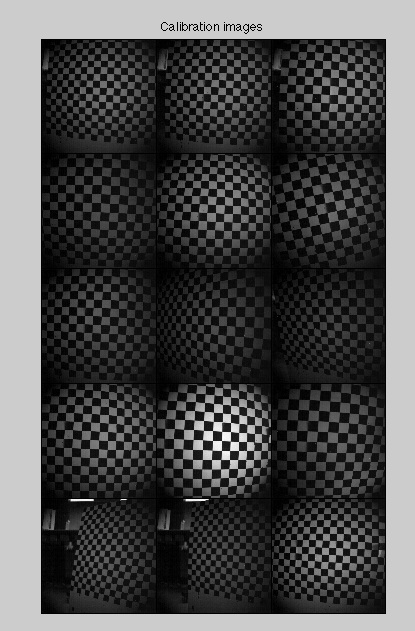
[[Image:CalibImages.jpg|thumb|500px|Mosaic of Calibration Images|left]] |
|||
[[Image:ErrorPlot.jpg]] |
|||
[[Image:ErrorPlot.jpgthumb|500px|Error Plot following optimization|right]] |
|||
Revision as of 16:44, 5 June 2010
Calibrating the High Speed Camera
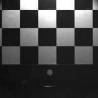
Before data can be collected from the HSV system, it is critical that the high speed camera be properly calibrated. In order to obtain accurate data, there is a series of intrinsic and extrinsic parameters that need to be taken into account. Intrinsic parameters include image distortion due to the camera itself, as shown in Figure 1. Extrinsic parameters account for any factors that are external to the camera. These include the orientation of the camera relative to the calibration grid as well as any scalar and translational factors.
In order to calibrate the camera, download the Camera Calibration Toolbox for Matlab. This resource includes detailed descriptions of how to use the various features of the toolbox as well as descriptions of the calibration parameters.
Once downloaded, to open the gui in matlab, go to the toolbox directory then type 'calib_gui' in the command window. (Then select standard memory).
For Tracking Objects in 2D
To calibrate the camera to track objects in a plane, first create a calibration grid. The Calibration Toolbox includes a calibration template of black and white squares of side length = 3cm. Print it off and mount it on a sheet of aluminum, foam core board or PVC to create a stiff backing. This grid must be as flat and uniform as possible to obtain an accurate calibration.
Intrinsic Parameters
Following the model of the first calibration example on the Calibration Toolbox website, use the high speed camera to capture 10-20 images, holding the calibration grid at various orientations relative to the camera. 1024x1024 images can be obtained using the "Moments" program. The source code can be checked out here.
Calibration Tips:
- One of the images must have the calibration grid in the tracking plane. This image is necessary for calculating the extrinsic parameters and will also be used for defining your origin.
- The images must be saved in the same directory as the Calibration Toolbox.
- Images must be saved under the same name, followed by the image number. (image1.jpg, image2.jpg...)
- The first calibration example on the Calibration Toolbox website uses 20 images to calibrate the camera. I have been using 12-15 images because sometimes the program is incapable of optimizing the calibration parameters if there are too many constraints.
- If a matlab error is generated before the calibration is complete, calibration will be lost. To prevent this, calibrate a set of images, then add groups of images to this set. To do this use the Add/Suppress Image feature. (Described in the 'first example' link above)
The Calibration Toolbox can also be use to compute the undistorted images as shown in Figure 2.
After entering all the calibration images, the Calibration Toolbox will calculate the intrinsic parameters, including focal length, principal point, and undistortion coefficients. There is a complete description of the calibration parameters here.
Extrinsic Parameters
In addition, the Toolbox will calculate rotation matrices for each image (saved as Rc_1, Rc_2...). These matrices reflect the orientation of the camera relative to the calibration grid for each image.
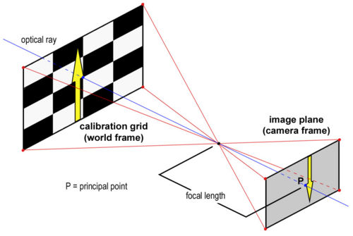
Figure 3 is an illustration of the pinhole camera model that is used for camera calibration. Since the coordinates of an object captured by the camera are reported in terms of pixels (camera frame), these data have to be converted to metric units (world frame).
In order to solve for the extrinsic parameters, first use the 'normalize' function provided by the calibration toolbox:
[xn] = normalize(x_1, fc, cc, kc, alpha_c);
where x_1 is a matrix containing the coordinates of the extracted grid corners in pixels for image1. The normalize function will apply any intrinsic parameters and return the (x,y) point coordinates free of lens distortion. These points will be dimensionless as they will all be divided by the focal length of the camera. Next, change the [2xn] matrix of points in (x,y) to a [3xn] matrix of points in (x,y,z) by adding a row of all ones. xn should now look something like this:
Where x_c, y_c, z_c, denote coordinates in the camera frame. z_c = focal length of the camera as calculated by the Calibration Toolbox.
Then, apply the rotation matrix, Rc_1:
[xn] = Rc_1*x_n;
We now have a matrix of dimensionless coordinates describing the location of the grid corners after accounting for distortion and camera orientation. What remains is to apply scalar and translational factors to convert these coordinates to the world frame. To do so, we have the following equations:
Where:
X_1 is the matrix containing the real world coordinates of the grid corners and is provided by the Calibration Toolbox. Cast these equations into a matrix equation of the form:
Where:
Finally, use the Matlab backslash command to compute the least squares approximation for the parameters S1, S2, T1, T1:
x = A\b
Now that all the parameters have been calculated, percentage error can be calculated, by applying the entire transformation process to the x_1 matrix and comparing the results to the X_1 matrix. If carefully executed, this calibration method can yield percent errors as low as 0.01%.
For Tracking Objects in 3D
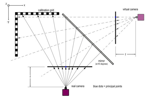
In order to obtain the coordinates of an object in three dimensions, a mirror can be used in order to create a "virtual camera," as shown in Figure 4.
Calibrating the camera to work in three dimensions is very similar to the two dimensional calibration. The main difference is the calibration grid itself. Instead of using a single flat plane for the calibration grid, an additional grid has to be constructed, consisting of two planes at 90 degrees as shown in the figure. This grid must be visible by both the "real" and "virtual" cameras. The purpose of this is to create a common origin. Having a common origin for both cameras will become critical in calculating an object's position in three dimensions.
Follow the steps for the 2D calibration and complete a separate calibration for each camera. The two sets of intrinsic parameters that are obtained should be identical in theory. In practice, they are likely to differ slightly.
Once the real world coordinates of an object in the XZ and YZ planes are obtained, the 3D position of the object still has to be obtained. The raw data is inaccurate because it represents the projection of the object's position onto the calibration plane. For the methodology and code required to execute these calculations, refer to the section entitled "Calculating the Position of an Object in 3D."
Using the High Speed Vision System
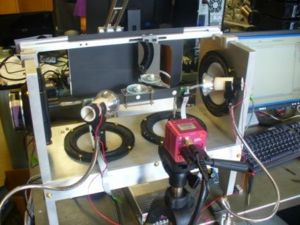
Figure 5 shows the current setup for the high speed vision system. The high speed camera is mounted on a tripod. The three lights surrounding the setup are necessary due to the high frequency with which the images are taken. The resulting camera shutter time is very small, so it is important to provide lots of light. The high frequency performance also has to be taken into consideration when processing the images. Processing one thousand 1024x1024 pixel images in real time proves impossible as well as unnecessary. The accompanying C program works by selection one or several regions of interest to focus on. The program applies a threshold to these regions. It then calculates an area centroid based off of the number of white pixels and re-centers the region of interest by locating the boundaries between the white and black pixels. The complete code for this program can be found here.
I will include a brief description of some of the important constants, which can be found in the header file 'constants.h'
EXPOSURE & FRAME_TIME: These parameters control number of images to be taken in one second, and are measured in microseconds. Frame time is the amount of time required to take on image. Exposure time is the amount of time the camera shutter is open, and should always be less than the frame time. A ratio of 5:2, FRAME:EXPOSURE seems to work well. To run the camera at 1000images/s for example, EXPOSURE and FRAME_TIME should be set to 400 and 1000, respectively.
SEQ & SEQ_LEN: For multiple regions of interest, the sequence describes the order in which the regions of interest are addressed. The current setup has the program cycling through the regions in order, so for 1000Hz with two regions, each region would have a frequency for 500images/s, and the camera would alternate between the two regions. For such a setup, SEQ would be set to {ROI_0, ROI_1} and SEQ_LEN set to 2.
INITIAL_BLOB_XMIN, INITIAL_BLOB_YMIN, INITIAL_BLOB_WIDTH, INITIAL_BLOB_HEIGHT: These parameters describe the initial position and size of the blob surrounding your object of interest. These should be set such that the blob surrounds the initial position of the object.
THRESHOLD: The threshold is the value (0-255) which is the cutoff value for the black/white boundary. The threshold will have to be adjusted depending on ambient light and the exposure time. It should be set such that the object of interest or fiduciary marker is in the white realm while everything in the background becomes black.
DISPLAY_TRACKING: This quantity should always be set to one or zero. When equal to one, it displays the region or regions of interest. This is convenient for setting the threshold and positioning the blobs. While taking data, however, this should be disabled in order to speed up the program.
DTIME: This value is the number of seconds of desired data collection. In order to collect data, run the program, wait for it to initialize, and then press 'd'. 'q' can be pressed at any time to exit the program.
Post-Processing of Data
Calculating the Position of an Object in 3D: Mathematical Theory
By comparing the data captured by the "real" camera and the "virtual" camera, it is possible to triangulate the three dimensional position of an object. The calibration procedures discussed earlier provide the real world (x,y) coordinates of any object, projected onto the calibration plane. By determining the fixed location of the two cameras, it is possible to calculate two position vectors and then compute a least squares approximation for their intersection.
The Calibration Toolbox provides the principal point for each camera measured in pixels. The principal point is defined as the (x,y) position where the principal ray (or optical ray) intersects the image plane. This location is marked by a blue dot in Figure 4. The principal point can be converted to metric by applying the intrinsic and extrinsic parameters discussed in the section "Calibrating the High Speed Camera."
From here, the distance from the cameras to the origin can be determined from the relationship:
Once this distance is calculated, the parallel equations can be obtained for a line in 3D with 2 known points:
Which can be rearranged in order to obtain 3 relationships:
These equations can be cast into matrix form:
There should be one set of equations for each vector, for a total of six equations. A should be a [6x3] matrix, and b should be a vector of length 6. Computing A\b in Matlab will yield the least squares approximation for the intersection of the two vectors.
% The function "calc_coords" takes as inputs, the raw data for vision in
% the XZ and XY planes.

% CC_xz and CC_yz are vectors of size [2x1] containing the principal points
% for each vision plane. Coordinates for principal point should be computed beforehand and reported in
% metric.

% FC_xz and FC_yz are vectors of size [2x1] containing the two focal
% lengths of the lens for each vision plane. These are obtained from the
% Calibration Toolbox and should be left in pixels.

% The function returns a matrix of size [nx3] containing the least squares
% approximation of the (x,y,z) coordinates based off of the vectors from
% the two cameras.

% NOTES:
% - All computations are done in metric. (Based off of calibration grid)
% - The XZ vision plane = "Real Camera"
% - The YZ vision plane = "Virtual Camera"

function XYZ = calc_coords(XZ, YZ, CC_xz, CC_yz, FC_xz, FC_yz);
matSize_xz = size(XZ);
num_datapoints_xz = matSize_xz(1,1);
matSize_yz = size(YZ);
num_datapoints_yz = matSize_yz(1,1);
num_datapoints = min(num_datapoints_xz, num_datapoints_yz);
XYZ = zeros(num_datapoints-1, 4);  % Initialize destination matrix
conv_xz = 5.40;  % Conversion factor (number of pixels / mm) for vision in XZ
conv_yz = 3.70;  % Conversion factor (number of pixels / mm) for vision in YZ
dist_origin_xz = [(FC_xz(1,1) + FC_xz(2,1)) / 2] / [conv_xz];   % Taking an average of the two focal lengths,
dist_origin_yz = [(FC_yz(1,1) + FC_yz(2,1)) / 2] / [conv_yz];       % Multiplying by conversion factor to get
                                                                        % the distance to the calibration grid in metric.
prinP_xz = [CC_xz(1,1); -dist_origin_xz; CC_xz(2,1)];         % [3X1] vector containing the coordinates of the principal points
prinP_yz = [dist_origin_yz; -CC_yz(1,1); CC_yz(2,1)];             % for the "Real" and "Virtual" Cameras.
for i = [1 : 1 : num_datapoints - 1]
    planeP_xz = [XZ(i,3); 0; XZ(i,4)];   % [3x1] vector containing the points in the plane of the calibration grid
    planeP_yz = [0; -(YZ(i+1,3)+YZ(i,3))/2; (YZ(i+1,4)+YZ(i,4))/2];
    x1_xz = prinP_xz(1,1);
    y1_xz = prinP_xz(2,1);
    z1_xz = prinP_xz(3,1);
    x1_yz = prinP_yz(1,1);
    y1_yz = prinP_yz(2,1);
    z1_yz = prinP_yz(3,1);
    x2_xz = planeP_xz(1,1);
    y2_xz = planeP_xz(2,1);
    z2_xz = planeP_xz(3,1);
    x2_yz = planeP_yz(1,1);
    y2_yz = planeP_yz(2,1);
    z2_yz = planeP_yz(3,1);
    % Set up matrices to solve matrix equation Ac = b, where c = [x, y, z]
    A_xz = [ (y2_xz - y1_xz), (x1_xz - x2_xz), 0;
        (z2_xz - z1_xz), 0, (x1_xz - x2_xz);
        0, (z2_xz - z1_xz), (y1_xz-y2_xz) ];
    b_xz = [ x1_xz*(y2_xz - y1_xz) + y1_xz*(x1_xz - x2_xz);
        x1_xz*(z2_xz - z1_xz) + z1_xz*(x1_xz - x2_xz);
        y1_xz*(z2_xz - z1_xz) + z1_xz*(y1_xz - y2_xz) ];
    A_yz = [ (y2_yz - y1_yz), (x1_yz - x2_yz), 0;
        (z2_yz - z1_yz), 0, (x1_yz - x2_yz);
        0, (z2_yz - z1_yz), (y1_yz-y2_yz) ];
    b_yz = [ x1_yz*(y2_yz - y1_yz) + y1_yz*(x1_yz - x2_yz);
        x1_yz*(z2_yz - z1_yz) + z1_yz*(x1_yz - x2_yz);
        y1_yz*(z2_yz - z1_yz) + z1_yz*(y1_yz - y2_yz) ];
    A = [A_xz; A_yz];
    b = [b_xz; b_yz];
    c = A\b;  % Solve for 3D coordinates
    XYZ(i, 1) = XZ(i,2);
    XYZ(i, 2) = c(1,1);
    XYZ(i, 3) = c(2,1);
    XYZ(i, 4) = c(3,1);
end
Calculating the Position of an Object on a Plane: Using Matlab
Similar to the above discussion, a point in 3D space can be determined (in world coordinates) based on the intrinsic and extrinsic parameters from calibration with a MatLab function. (It is assumed the Z value is a plane and is a constant known parameter)
[World_x, World_y] = Transpose(Rc_ext) * (zdist_pix *(normalize([pix_x, pix_y], fc, cc, kc, alpha_a), 1) - Tc_ext)
Where: Rc_Ext and Tc_ext are parameters from the extrinsic calibration zdist_pix is the distance from the focal point to the object in pixels. (measure distance from camera to object using meter stick then convert to pixels by determining the number of pixels per cm in calibration image at that distance) pix_x and pix_y are the camera pixel coordinates corresponding to the desired world point fc, cc, kc and alpha_a are parameters from the intrinsic camera calibration
Finding Maxes and Mins, Polyfits
The following Matlab function was used to calculate the minima of a set of data:
% Function locates the minima of a function, based on the 3 previous and
% 3 future points.
% Function takes one input, an [nx4] matrix where:
% ydisp(1,:) = image number from which data was taken.
% ydisp(2,:) = time at which data was taken.
% ydisp(3,:) = x or y position of object.
% ydisp(4,:) = z position (height of object).
% The function returns a matrix of size [nx3] containing the image number,
% time, and value of each local minimum.
function Mins = calc_minima(ydisp);
Mins = zeros(10, 3);
mat_size = size(ydisp);
num_points = mat_size(1,1);
local_min = ydisp(1, 4);
time = ydisp(1, 1);
location = 1;
index = 1;
min_found = 0;
for i = [4 : 1 : num_points - 3]
    % execute if three previous points are greater in value
    if ( ydisp(i, 4) < ydisp(i - 1, 4) && ydisp(i, 4) < ydisp(i - 2, 4) && ydisp(i, 4) < ydisp(i - 3, 4))
        local_min = ydisp(i, 4);
        time = ydisp(i, 1);
        location = i;
        % if next three points are also greater in value, must be a min
        if ( ydisp(i, 4) < ydisp(i + 1, 4) && ydisp(i, 4) < ydisp(i + 2, 4) && ydisp(i, 4) < ydisp(i + 3, 4))
            min_found = 1;
        end
    end
    if (min_found)
        Mins(index, 1) = location;
        Mins(index, 2) = time;
        Mins(index, 3) = local_min;
        index = index + 1;
        min_found = 0;
    end
 end
Once the minima were located, the following was used to compute a second order polyfit between two consecutive minima:
% plot_polyfit calls on the function calc_minima to locate the local mins
% of the data, and then calculates a parabolic fit in between each of two
% consecutive minima.
% It takes in raw_data in the form of an [nx4] matrix and returns
% a matrix containing the fitted data, the matrix of calculated minima, and
% the matrix of calculated maxima.
function [fittedData, Maxima, Mins] = plot_polyfit(raw_data);
num_poly = 2;
timestep = 1000;
fittedData = zeros(100,3);
Mins = calc_minima(raw_data);    % Calculate minima
Maxima = zeros(10,2);
mat_size = size(Mins);
num_mins = mat_size(1,1);
index = 1;
max_index = 1;
% For each min, up until the second to last min, execute the following...
for i = [1 : 1 : num_mins - 1]
    % Calculate coefficients, scaling, and translational factors for polyfit
    [p,S,mu] = polyfit(raw_data(Mins(i, 1) : Mins(i+1, 1), 2), raw_data(Mins(i, 1) : Mins(i+1, 1), 4), num_poly);
    start = index;
    % Given the parameters for the polyfit, compute the values of the
    % function for (time at first min) -> (time at second min)
    for time = [raw_data(Mins(i, 1), 2) : timestep : raw_data(Mins(i + 1, 1), 2)]
        fittedData(index, 1) = time;
        x = [time - mu(1,1)] / mu(2,1);
        y = 0;
        v = 0;
        % For each term in the polynomial
        for poly = [1 : 1 : num_poly + 1]
            y = y + [ p(1, num_poly - poly + 2) ]*x^(poly-1);
            v = v + (poly-1)*[ p(1, num_poly - poly + 2) ]*x^(poly-2);
        end
        fittedData(index, 2) = y;
        fittedData(index, 3) = v;
        index = index + 1;
    end
    t = -p(1,2)/(2*p(1,1));
    x = [t * mu(2,1)] + mu(1,1);
    local_max = 0;
    for poly = [1 : 1 : num_poly + 1]
        local_max = local_max + [ p(1, num_poly - poly + 2) ]*t^(poly-1);
    end
    Maxima(max_index, 1) = x;
    Maxima(max_index, 2) = local_max;
    max_index = max_index + 1;
end
Error Minimization of Calibration Coefficients
Following the computation of the intrinsic parameters, the relative error can be analyzed using the calibration toolbox. To see the error in a graphical form click 'Analyze Error' in the main gui. This plot will show the error in pixel units. The different point colors represent different images used for calibration. To begin to optimize this error, click on an outlier point. The image number and point of this point will be displayed in the matlab command window. Click outliers of the same color, is there a specific image that has many errors?
You can also view the projected calibration points on a specific image by clicking 'Reproject on Image' and at the prompt enter the number of the error prone image. This will allow you to see the points which are creating the most error. If the calibration points are significantly off the corners of the grid, it may be a good idea to use 'Add/Suppress Images' to remove then recalibrate the image. (You can also click all corners manually)
However, if the entire image is not error prone, it is possible to minimize the error by changing the dimensions of the "search box" for which the calibration algorithm looks for a corner. This is accomplished by changing the values of wintx and winty, the default values during calibration are set at 5. To do this click 'Recomp Corners' in the calibration gui, then at the prompt for wintx and winty enter a different (typically larger value, ie 8). Then at the prompt for the numbers of the images for which to recompute the corners, enter the numbers of the images with the error outliers as determined above.
Repeat this process until the error is within reason. (Typically 3-4 pixels, but dependent on resolution, distance from object, pixel size and application)
Further information and examples can be found at the first calibration example.
Example Intrinsic Parameters (LIMS Lab, Winter 2010)
The below example was completed for the high speed vision system in the LIMS lab during Winter Quarter 2010.
Number of Images = 15
Error optimization completed by adjusting the values of winty and wintx for various images.
Calibration results after optimization (with uncertainties):
Focal Length: fc = [ 1219.49486 1227.09415 ] ± [ 1.98092 1.95916 ] Principal point: cc = [ 502.28854 524.25824 ] ± [ 1.26522 1.07298 ] Skew: alpha_c = [ 0.00000 ] ± [ 0.00000 ] => angle of pixel axes = 90.00000 ± 0.00000 degrees Distortion: kc = [ -0.39504 0.36943 -0.00018 -0.00105 0.00000 ] ± [ 0.00307 0.01033 0.00016 0.00021 0.00000 ] Pixel error: err = [ 0.27578 0.25400 ]
Note: The numerical errors are approximately three times the standard deviations (for reference).

