High Speed Vision System and Object Tracking

Last modified 6 June, 2009

Calibrating the High Speed Camera

Figure 1: Calibration grid with distortion.

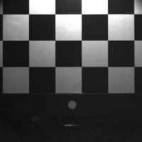
Before data can be collected from the HSV system, it is critical that the high speed camera be properly calibrated. In order to obtain accurate data, there is a series of intrinsic and extrinsic parameters that need to be taken into account. Intrinsic parameters include image distortion due to the camera itself, as shown in Figure 1. Extrinsic parameters account for any factors that are external to the camera. These include the orientation of the camera relative to the calibration grid as well as any scalar and translational factors.

In order to calibrate the camera, download the Camera Calibration Toolbox for Matlab. This resource includes detailed descriptions of how to use the various features of the toolbox as well as descriptions of the calibration parameters.

For Tracking Objects in 2D

To calibrate the camera to track objects in a plane, first create a calibration grid. The Calibration Toolbox includes a calibration template of black and white squares of side length = 3cm. Print it off and mount it on a sheet of aluminum or PVC to create a stiff backing. This grid must be as flat and uniform as possible in order to obtain an accurate calibration.

Intrinsic Parameters

Following the model of the first calibration example on the Calibration Toolbox website, use the high speed camera to capture 10-20 images, holding the calibration grid at various orientations relative to the camera. 1024x1024 images can be obtained using the "Moments" program. The source code can be checked out here.

Figure 2: Calibration grid undistorted.

Calibration Tips:

• One of the images must have the calibration grid in the tracking plane. This image is necessary for calculating the extrinsic parameters and will also be used for defining your origin.
• The images must be saved in the same directory as the Calibration Toolbox.
• Images must be saved under the same name, followed by the image number. (image1.jpg, image2.jpg...)
• The first calibration example on the Calibration Toolbox website uses 20 images to calibrate the camera. I have been using 12-15 images because sometimes the program is incapable of optimizing the calibration parameters if there are too many constraints.

The Calibration Toolbox can also be use to compute the undistorted images as shown in Figure 2.

After entering all the calibration images, the Calibration Toolbox will calculate the intrinsic parameters, including focal length, principal point, and undistortion coefficients. There is a complete description of the calibration parameters here.

Extrinsic Parameters

In addition, the Toolbox will calculate rotation matrices for each image (saved as Rc_1, Rc_2...). These matrices reflect the orientation of the camera relative to the calibration grid for each image.

Figure 3: Projection of calibration grid onto the image plane.

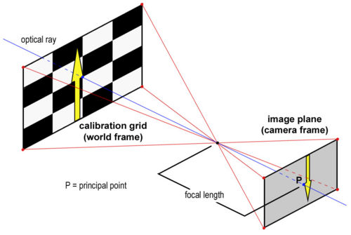
Figure 3 is an illustration of the pinhole camera model that is used for camera calibration. Since the coordinates of an object captured by the camera are reported in terms of pixels (camera frame), these data have to be converted to metric units (world frame).

In order to solve for the extrinsic parameters, first use the 'normalize' function provided by the calibration toolbox:

  [xn] = normalize(x_1, fc, cc, kc, alpha_c);

where x_1 is a matrix containing the coordinates of the extracted grid corners in pixels for image1. The normalize function will apply any intrinsic parameters and return the (x,y) point coordinates free of lens distortion. These points will be dimensionless as they will all be divided by the focal length of the camera. Next, change the [2xn] matrix of points in (x,y) to a [3xn] matrix of points in (x,y,z) by adding a row of all ones. xn should now look something like this:

$\mathbf {xn} ={\begin{bmatrix}x_{c}1/z_{c}&x_{c}2/z_{c}&...&x_{c}n/z_{c}\\y_{c}1/z_{c}&y_{c}2/z_{c}&...&y_{c}n/z_{c}\\z_{c}/z_{c}&z_{c}/z_{c}&...&z_{c}/z_{c}\end{bmatrix}}$ Where xc, yc, zc, denote coordinates in the camera frame. zc = focal length of the camera as calculated by the Calibration Toolbox.

Then, apply the rotation matrix, Rc_1:

  [xn] = Rc_1*x_n;

We now have a matrix of dimensionless coordinates describing the location of the grid corners after accounting for distortion and camera orientation. What remains is to apply scalar and translational factors to convert these coordinates to the world frame. To do so, we have the following equations:

$X_{1}(1,1)=S1*xn(1,1)+T1\,$

$X_{1}(2,1)=S2*xn(2,1)+T2\,$