Difference between revisions of "Bouncing Polygon Simulator"
| (54 intermediate revisions by the same user not shown) | |||
| Line 3: | Line 3: | ||
The polygon simulator program files model an object (ball or polygon) bouncing on a flat surface. It works by iterating through the object's flight trajectory one time step at a time. If the program finds that the object is below the contact surface after a time step then the program will use a zerofinder to compute the exact time (to a tolerance) when the object contacts the surface. After finding each impact time, the program uses an impact model to compute the post-impact state of the object. The object then continues on a new flight trajectory based on the post-impact states found by the impact model and the process repeats itself. |
The polygon simulator program files model an object (ball or polygon) bouncing on a flat surface. It works by iterating through the object's flight trajectory one time step at a time. If the program finds that the object is below the contact surface after a time step then the program will use a zerofinder to compute the exact time (to a tolerance) when the object contacts the surface. After finding each impact time, the program uses an impact model to compute the post-impact state of the object. The object then continues on a new flight trajectory based on the post-impact states found by the impact model and the process repeats itself. |
||
The program has some limitations. For instance, it can't model an object resting on a surface. This means that every time the surface "catches" the object, the program breaks down. The error printed out is "dt = 0: exiting simulation". This error does not always correspond to the surface catching the object. Literally it means that the zerofinder was converging on a zero time step. This would cause the object to never step forward in time, which is why the program exits if this happens. Another limitation is the impact model. The program can only simulate an impact of one vertex contact. In other words, the object cannot contact the surface with two vertices simultaneously. |
The program has some limitations. For instance, it can't model an object resting on a surface. This means that every time the surface "catches" the object, the program breaks down. The error printed out is "dt = 0: exiting simulation". This error does not always correspond to the surface catching the object. Literally it means that the zerofinder was converging on a zero time step. This would cause the object to never step forward in time, which is why the program exits if this happens. Another limitation is the impact model. The program can only simulate an impact of one vertex contact. In other words, the object cannot contact the surface with two vertices simultaneously. The programs prints out "multiple points of contact", but does not exit the simulation; the program continues running. |
||
'''''You can download the polygon simulator codes''''' [[media:SimulationCodes.zip|'''''here''''']]. |
|||
=Run a simulation and watch a movie= |
|||
=Run A Simulation And Watch A Movie= |
|||
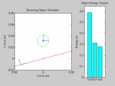
There are three ways to run a simulation. You can run the simulation for a certain amount of time and watch the movie while the simulation is running (option 1). This option is not recommended because it slows down the simulation and the movie lags a lot. Another way is to run the simulation for a certain amount of time and then construct a movie afterwards. The last way is to run the simulation for a certain number of impacts and post-construct the movie. |
There are three ways to run a simulation. You can run the simulation for a certain amount of time and watch the movie while the simulation is running (option 1). This option is not recommended because it slows down the simulation and the movie lags a lot. Another way is to run the simulation for a certain amount of time and then construct a movie afterwards. The last way is to run the simulation for a certain number of impacts and post-construct the movie. |
||
| Line 16: | Line 18: | ||
**object.r - defines the radius of a ball. The user may enter any value for this if the object is a polygon. |
**object.r - defines the radius of a ball. The user may enter any value for this if the object is a polygon. |
||
**object.theta - defines the original angle of each vertex in relation to the center of mass. The user does not have to enter this variable. |
**object.theta - defines the original angle of each vertex in relation to the center of mass. The user does not have to enter this variable. |
||
[[image:SimulatorViewer.jpg|thumb|400px|Simulation Viewer|right]] |
|||
**object.inertia - defines the inertia of the object. The user must enter this. |
**object.inertia - defines the inertia of the object. The user must enter this. |
||
**object.u - defines the friction coefficient between the ball and the table. |
**object.u - defines the friction coefficient between the ball and the table. |
||
| Line 60: | Line 63: | ||
*Once the simulation has finished running, the user may construct a movie if they chose option 2 or 3. |
*Once the simulation has finished running, the user may construct a movie if they chose option 2 or 3. |
||
F = movconstr(contstates,table,params,object); |
F = movconstr(contstates,table,params,object,t0,t1); |
||
inputs: |
|||
1) contstates, table, and object are all outputs from the polysim function |
|||
2) params is the input used in the polysim function |
|||
3) t0 & t1 specify the time range for the movie if you want to watch what happens during the simulation from t0 to t1 |
|||
outputs: |
|||
1) F is an array of frames that may be used to construct a movie. |
1) F is an array of frames that may be used to construct a movie. |
||
*The user may then convert the set of frames, F, into an avi file. |
*The user may then convert the set of frames, F, into an avi file. Matlab can output in the following formats: |
||
(Indeo3, Indeo5, Cinepak, MSVC, RLE) |
|||
As far as I've looked, there are no codecs available for Mac OSX to convert from these formats. The movies play fine on the Windows Media Player though. |
|||
movie2avi(‘filename.avi’,F); |
movie2avi(‘filename.avi’,F); |
||
NOTE: Sample simulations are attached to the end of the polysim.m code. |
NOTE: Sample simulations are attached to the end of the polysim.m code. |
||
=Running Simulations Without The Symbolic Toolbox= |
|||
The symbolic toolbox is used within the polysim.m program to take the derivatives of the table functions entered by the user. If you don't have the symbolic toolbox, this just means you have to define the derivatives (table.xd, table.yd, table.phid) manually before you run a simulation. All you need to do is change the lines starting at line 107 in the polysim.m code as follows: |
|||
table.xd = inline(char(diff(table.x))); ----> table.xd = inline(table.xd); |
|||
table.yd = inline(char(diff(table.y))); ----> table.yd = inline(table.yd); |
|||
table.phid = inline(char(diff(table.phi))); ----> table.phid = inline(table.phid); |
|||
Remember you must manually specify table.xd, table.yd, and table.phid just as you would define table.x, table.y, and table.phid before running a simulation. |
|||
Example: |
|||
table.x = '0'; |
|||
table.y = '5*sin(2*t)+3'; |
|||
table.phi = '0'; |
|||
table.xd = '0'; |
|||
table.yd = '10*cos(2*t)'; |
|||
table.phid = '0'; |
|||
=Bifurcation Diagrams / Long Time Behavior Plots= |
=Bifurcation Diagrams / Long Time Behavior Plots= |
||
| Line 77: | Line 113: | ||
state.y = [num2str(lam(ii)),’*1e-2’]; |
state.y = [num2str(lam(ii)),’*1e-2’]; |
||
[[image:BifDiag_Small.jpg|thumb|350px|Sample Bifurcation Diagram|right]] |
|||
Then specify lambda, the drop height range, which is in multiples of 1 cm. |
Then specify lambda, the drop height range, which is in multiples of 1 cm. |
||
The program returns lam, hmax, xpos, vpost, and time. |
The program returns lam, hmax, xpos, vpost, and time. |
||
| Line 92: | Line 131: | ||
5) time is the time it took to run the bifDiagram program |
5) time is the time it took to run the bifDiagram program |
||
NOTE: A sample simulation is attached at the end of the bifDiagram.m code. |
NOTE: A sample simulation is attached at the end of the bifDiagram.m code. |
||
=Trajectory / TrajectoryANDTable= |
=Trajectory / TrajectoryANDTable= |
||
| Line 100: | Line 144: | ||
[t,x,y] = trajectory(contstates,step,t0,t1); |
[t,x,y] = trajectory(contstates,step,t0,t1); |
||
[t,x,y,tx,ty] = trajectoryANDTable(contstates,step,t0,t1,table); |
|||
[[image:Period1Traj.jpg|thumb|350px|Period-1 Trajectory|right]] |
|||
Input: |
Input: |
||
| Line 110: | Line 157: | ||
4) t1 is the end point for the data construction |
4) t1 is the end point for the data construction |
||
Output: |
|||
1) t is a vector containing the times |
|||
2) x (y) contains the x (y) position of the object |
|||
4) tx (ty) contains the x (y) position of the table |
|||
=Period1= |
=Period1= |
||
[[image:Period1Stab.jpg|thumb|350px|Stable Period-1 Orbit|left]][[image:Period1Unstab.jpg|thumb|350px|Unstable Period-1 Orbit|right]] |
|||
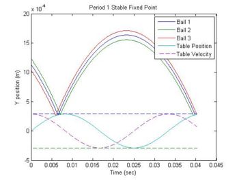
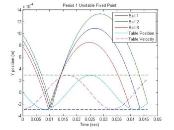
Period1 plots the trajectory of a ball around its period 1 fixed points. It plot three trajectories. One is the the ball exactly at its fixed point. The other two are at points before and after the fixed point. |
Period1 plots the trajectory of a ball around its period 1 fixed points. It plot three trajectories. One is the the ball exactly at its fixed point. The other two are at points before and after the fixed point. |
||
If the user wants to change from viewing the plot of a stable fixed point to an unstable fixed point or vice versa, reverse the sign of variable A (table amplitude) in line 12 of the period1.m code. |
|||
=Functions Used By These Programs= |
=Functions Used By These Programs= |
||
Latest revision as of 21:13, 16 June 2009
Overview
The polygon simulator program files model an object (ball or polygon) bouncing on a flat surface. It works by iterating through the object's flight trajectory one time step at a time. If the program finds that the object is below the contact surface after a time step then the program will use a zerofinder to compute the exact time (to a tolerance) when the object contacts the surface. After finding each impact time, the program uses an impact model to compute the post-impact state of the object. The object then continues on a new flight trajectory based on the post-impact states found by the impact model and the process repeats itself.
The program has some limitations. For instance, it can't model an object resting on a surface. This means that every time the surface "catches" the object, the program breaks down. The error printed out is "dt = 0: exiting simulation". This error does not always correspond to the surface catching the object. Literally it means that the zerofinder was converging on a zero time step. This would cause the object to never step forward in time, which is why the program exits if this happens. Another limitation is the impact model. The program can only simulate an impact of one vertex contact. In other words, the object cannot contact the surface with two vertices simultaneously. The programs prints out "multiple points of contact", but does not exit the simulation; the program continues running.
You can download the polygon simulator codes here.
Run A Simulation And Watch A Movie
There are three ways to run a simulation. You can run the simulation for a certain amount of time and watch the movie while the simulation is running (option 1). This option is not recommended because it slows down the simulation and the movie lags a lot. Another way is to run the simulation for a certain amount of time and then construct a movie afterwards. The last way is to run the simulation for a certain number of impacts and post-construct the movie.
Before you run a simulation, you must specify the ball-table system.
- Object – defines the the polygon/ball
- object.nvert - is 1 for a ball and the number of vertices for a polygon.
- object.x - defines the x coordinates of the center of mass and vertices of the polygon or ball. If the object is a ball, all that is needed is the centroid of the ball. If the object is a polygon, the user must enter a vector whose first entry is the centroid and succesive entries are the vertices of the polygon.
- object.y - defines the y coordinates of the polygon in the same way.
- object.r - defines the radius of a ball. The user may enter any value for this if the object is a polygon.
- object.theta - defines the original angle of each vertex in relation to the center of mass. The user does not have to enter this variable.
- object.inertia - defines the inertia of the object. The user must enter this.
- object.u - defines the friction coefficient between the ball and the table.
- object.res - defines the restitution coefficient between the ball and the table.
- State – defines the initial state of the polygon/ball
- state.x - defines the initial x position of the center of mass.
- state.y - defines the initial y position of the center of mass.
- state.theta - defines the initial theta position of the ball/polygon with respect to object.theta
- state.xd - defines the initial x velocity of the center of mass.
- state.yd - defines the initial y velocity of the center of mass.
- state.thetad - defines the initial rotational velocity about the center of mass
- Table – defines the functions describing the table motion which are entered as strings.
- table.x - defines the x function for the table.
- table.y - defines the y function for the table.
- table.phi - defines the angle function for the table.
- table.xd - defines the x velocity function for the table. The user does not need to enter this unless they are using Matlab without the symbolic toolbox. There are instructions for this specific circumstance.
- table.yd - defines the y velocity function for the table and also requires the symbolic toolbox.
- table.phid - defines the angular velocity function for the table and requires the toolbox.
- Params – defines the miscellaneous parameters for running the simulation.
- params.step - defines the minimum step size to be used during the simulation.
- params.stepmov - defines the time step size for view a movie.
- params.T - defines how long to run the simulation for. The user may enter any value for this if they are using option 3.
- params.hitlim - defines how many table-ball impacts the program should simulate. The user may enter any value for this if they are using options 1 or 2.
- params.windim - defines the viewing window size for the movie. This is a vector that follows [xmin xmax ymin ymax].
- After the user has specified all the necessary information to describe the table-ball system, they may run the polysim function.
[F,contstates,object,table,steplist] = polysim(object,state,table,params,option);
1) F is an array of frames that may be used to construct a movie. F is an empty matrix if the user chose option 2 or 3.
2) contstates is a structure holding the times and object state at each impact.
- Contstates{1} = times
- Contstates{2} = impact states which are structures
3) object and table simply return the object and table given by the user
4) steplist returns the list of time steps used during the simulation
- Once the simulation has finished running, the user may construct a movie if they chose option 2 or 3.
F = movconstr(contstates,table,params,object,t0,t1);
inputs:
1) contstates, table, and object are all outputs from the polysim function
2) params is the input used in the polysim function
3) t0 & t1 specify the time range for the movie if you want to watch what happens during the simulation from t0 to t1
outputs:
1) F is an array of frames that may be used to construct a movie.
- The user may then convert the set of frames, F, into an avi file. Matlab can output in the following formats:
(Indeo3, Indeo5, Cinepak, MSVC, RLE)
As far as I've looked, there are no codecs available for Mac OSX to convert from these formats. The movies play fine on the Windows Media Player though.
movie2avi(‘filename.avi’,F);
NOTE: Sample simulations are attached to the end of the polysim.m code.
Running Simulations Without The Symbolic Toolbox
The symbolic toolbox is used within the polysim.m program to take the derivatives of the table functions entered by the user. If you don't have the symbolic toolbox, this just means you have to define the derivatives (table.xd, table.yd, table.phid) manually before you run a simulation. All you need to do is change the lines starting at line 107 in the polysim.m code as follows:
table.xd = inline(char(diff(table.x)));        ---->    table.xd = inline(table.xd);
table.yd = inline(char(diff(table.y)));        ---->    table.yd = inline(table.yd);
table.phid = inline(char(diff(table.phi)));    ---->    table.phid = inline(table.phid);
Remember you must manually specify table.xd, table.yd, and table.phid just as you would define table.x, table.y, and table.phid before running a simulation.
Example:
table.x = '0';
table.y = '5*sin(2*t)+3';
table.phi = '0';
table.xd = '0';
table.yd = '10*cos(2*t)';
table.phid = '0';
Bifurcation Diagrams / Long Time Behavior Plots
[lam,hmax,xpos,vpost,time] = bifDiagram(lam,object,state,table,params);
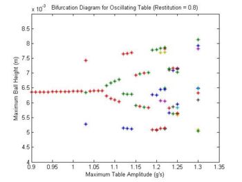
This program simulates multiple ball-table systems each for a certain number impacts. Each system is different based on parameters ranged by the user. Lam, “lambda”, is a vector containing these parameters. For example, if you want to look at how changing the drop height of the ball changes the long time behavior of the system, you open up bifDiagram.m and input the following at line 22.
state.y = [num2str(lam(ii)),’*1e-2’];
Then specify lambda, the drop height range, which is in multiples of 1 cm.
The program returns lam, hmax, xpos, vpost, and time.
1) lam is the same vector entered by the user
2) hmax is a matrix containing the maximum height the ball reaches in between each impact for every simulation run
- hmax(row,col): row – impacts, col – lamda values
3) xpos is a matrix containing the x position of the ball at each impact. The rows and columns behave the same way as hmax
4) vpost is a matrix containing the post impact velocities
5) time is the time it took to run the bifDiagram program
NOTE: A sample simulation is attached at the end of the bifDiagram.m code.
Trajectory / TrajectoryANDTable
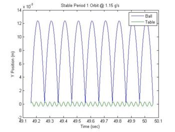
Both trajectory and trajectoryANDTable return the time evolution of the x and y position of the ball/polygon by reconstructing the data from impact states (contstates). The trajectoryANDTable program returns the the time evolution of the x and y position of the table as well.
[t,x,y] = trajectory(contstates,step,t0,t1);
[t,x,y,tx,ty] = trajectoryANDTable(contstates,step,t0,t1,table);
Input:
1) contstates is the same contstates variable that is returned from polysim program
2) step is the stepsize in between data points that you want the trajectory program to output
3) t0 is the starting point for the data construction
4) t1 is the end point for the data construction
Output:
1) t is a vector containing the times
2) x (y) contains the x (y) position of the object
4) tx (ty) contains the x (y) position of the table
Period1
Period1 plots the trajectory of a ball around its period 1 fixed points. It plot three trajectories. One is the the ball exactly at its fixed point. The other two are at points before and after the fixed point.
If the user wants to change from viewing the plot of a stable fixed point to an unstable fixed point or vice versa, reverse the sign of variable A (table amplitude) in line 12 of the period1.m code.
Functions Used By These Programs
1) zerofinder – A binary serach program that returns the table-ball impact times.
2) datarecon – reconstructs the objects flight data using pre and post imapact states as well as the movie step size specified by the user
3) polyplot – updates the plot frame with the current system state
4) impact – returns the object post impact state based on the system pre impact state
