Variable Frequency Electrosense

Introduction

INSERT INTRO

Team

• Tod Reynolds
• Pill Gun Park
• Joshua Peng

INSERT TEAM PIC

Code

Processing Code

The Processing code will display a window on the computer monitor that allows the user to control the motion of the linear actuator and sensor, run through a single routine of calculation and plotting, and run through full object identification and object detection routines.

INSERT PIC OF WINDOW

Buttons

Sensing Control

• Calibrate: returns the emitter/sensor board to the zero position. Unless it is in the middle of calculating and plotting, the board will immediately head in the reverse direction until it hits the limit switch and then it will go forward 200 steps so that the limit switch is completely released. All of our tests have been designed and analyzed according to and starting from this zero position. Once the Calibrate button is pushed, this process cannot be stopped unless someone flips the PIC power switch or the +12V/-12V power switch, etc.
• Activate: activates the linear actuator so that the board can move
• Data Acquisition: activates calculation and plotting (runs the Object Detection routine)
• Calculate/Plot: runs through a single routine of calculation and plotting, the board will not move after the bode plots are generated.

Linear Actuator Control

Note: for these buttons to have any effect, the "Activate" button needs to be pressed before these buttons

• Pause: board will stop moving (if it was already moving)
• Forward: board will move forward (if not already moving forward) at a constant speed
• Reverse: board will move reverse (if not already moving reverse) at a constant speed
• Accelerate: board will increase speed (by decreasing the delay between clock pulses of the bipolar stepper motor by 1 ms)
• Slow: board will decrease speed (by increasing the delay between clock pulses of the bipolar stepper motor by 1 ms)

Object Detection

• In order to run the Object Detection routine, you must press the "Data Acquisition" and "Activate" in sequence.
• "Data Acquisition" should be pressed first and "Activate" after. The board will then perform calculations and plotting at its current position, then move a halfinch forward, and then repeat this process until it hits the limit switch at the end.
• If you press "Activate" first, then "Data Acquisition" after, the board will move a halfinch forward from its current position, perform calculations and plotting after it stops, and then it will repeat this process until it hits the limit switch at the end. In this case, the step and location (according to the hashes) in the text file output will be off by 1 index.

Object Identification

• The Object Identification routine is performed automatically when "Data Acquisition" and "Activate" are pressed in sequence.
• Once the board has stopped moving and all 19 magnitude and phase bode plot points have been calculated and plotted, the program will compare the bode plot with library of bode plots of different object type in which the object was directly underneath the sensor and display the object index of the object with the closest matching bode plot for magnitude and phase in the space between the buttons.
• Thus, the program will try to identify whatever is underneath the sensor at its current position after each calculation and plotting routine (each time it has moved and stopped).

Window Contents

• Emitted and sensed sinusoidal signals plots - in the top left quadrant, these signals are plotted with horizontal guidelines that hit the maximum peak of the waves which also display the amplitude (mapped analog voltage values) so that you can visually compare and calculate the magnitude just by analyzing this plot. These signals also have vertical guidelines that hit the vertical mid point of both waves so that you can check the phase shift between the emitted and sensed waves. The amplitude difference and phase shift is displayed in the top corners of the plot.

• FFT Magnitude plot - the whole magnitude spectrum of the FFT of the emitted and sensed wave is plotted in the middle left quadrant. There are vertical guidelines showing the frequency at the peak for both the emitted and sensed wave and what it should be (the frequency of waves we are sending out of the AD9833 function generator chip). If the transfer function from the input (emitted wave) to the output (sensed wave) is linear, then there should only be a single peak in this plot.

• FFT Phase plot - the whole phase spectrum of the FFT of the emitted and sensed wave is plotted in the bottom left quadrant. The same vertical guidelines used in the FFT Magnitude plot are used here.

• Magnitude and Phase Bode plots - an experimental magnitude and phase bode plot is plotted at 19 frequencies between 100Hz and 10kHz

• Display of Object Type and Object Location - assuming that the sensor passes an object as it moves forward and runs through routines, program will run through an algorithm to determine where the object is according to the hashes on the back and what the object type is according to a bode plot library

• Space for data display and debugging - You can uncomment some portions of our code to display the values of arrays and variables on the empty right side of the window. Currently, for a few seconds after a calculation and plotting routine (until the board finishes moving a halfinch), the program will display the 19 magnitude and phase points of the bode plot. It also currently continuously displays many of the variables used in the calc() function.

Code

Description of Functions

Our full Processing code is much too long to post here, so we will instead post a link here and at the end of this section to a zip file with the actual code with comments. Some of the more important functions are posted. Please note that you need to install the "ControlP5" custom GUI element library for Processing 1.0 by Andreas Schlegel in order for this Processing program to work. The following section will describe what each function in our code does.

initserial()

Processing is set up so that it is continuously looking for data on the rs232 lines and once it sees data it will automatically start retrieving it. Once the sensor has finished moving and fully stopped, the pic will send 5 arrays each with 512 data points to Processing. The first set of arrays (data points) retrieved are of the 100 Hz voltage sinusoidal signals emitted and sensed. Next, there is a delay in the PIC, the sampling frequency is adjusted, the frequency of the signals is increased to 200 Hz, the fft of the signals is calculated, and then the next set of arrays corresponding to the 200 Hz wave is sent out and received by Processing. This process is repeated until it goes through all 19 frequencies (100 Hz, 200 Hz, 300 Hz,…,10 kHz).

• vector of frequencies (x axis) used to calculate the fft in the PIC, note that the first half (first 256 points) is nonzero, the second half is deleted (all zeros) in the PIC because it is essentially the same as the first half but in reverse order (256 frequency points + 256 zeros)

• y axis points of the emitted sinusoidal signal (512 emitted wave points)

• y axis points of the sensed sinusoidal signal (512 sensed wave points)

• real component of the complex values resulting from the fft of both emitted and sensed signals. First 256 points are of the emitted signal, second 256 points are of the sensed signal. (256 emitted wave points + 256 sensed wave points)

• imaginary component of the complex values resulting from the fft of both emitted and sensed signals. First 256 points are of the emitted signal, second 256 points are of the sensed signal. (256 emitted wave points + 256 sensed wave points)

• integer variable “finish” that corresponds to “halfinch” in the PIC code. (more on this below)

    // grab the data
    if ((line_received.length == 6) && (portNumber==0)){
      if (index >= L){
        index = 0;
        newdata = true;
        for (int i=0;i<L;i++) {
        sin1[i] = map(nsin1[i],min(nsin1)-300,max(nsin1)+300,-1*int(by*3/8),int(by*3/8));
        sin2[i] = map(nsin2[i],min(nsin2)-300,max(nsin2)+300,-1*int(by*3/8),int(by*3/8)); 
        }
      }
      freq[index] = line_received[0];
      nsin1[index] = line_received[1];
      nsin2[index] = line_received[2];
      real[index] = line_received[3];
      imag[index] = line_received[4];
      
      if (line_received[5] > finish) {
        kk = 0;
        reinitializebp();
        finish = int(line_received[5]);
      }
      index++;

• Note that we use this “newdata” Boolean variable to ensure that once we start collecting data points, we will finish collecting all 512 data points before we can use the data points for calculating and plotting in the other functions.

• The sin1[] and sin2{} arrays collect the mapped nsin1[] and nsin2[] values respectively. They are mapped according to the sine wave plotting window dimensions.

• There is a corresponding integer variable to “finish” called “halfinch” in the PIC code that counts the 37 half-inches that the sensor/emitter board can move along the water tank. It is incremented each time after the board moves a half-inch forward. Right after the PIC finishes moving that half-inch, it needs to tell Processing that it is ready to start fft calculation and will begin to send data points over by sending this incremented “halfinch.” Even though we just want to send “halfinch” over, when you send data via rs232, you must send all the information over. So the PIC will first send out dummy data points plus an incremented “halfinch”. It is compared to “finish,” “kk” is reset back to zero and the bode plots are cleared.

global variables and setup()

Some important variables:

• int kk = 0;

frequency counter, kk is incremented by 1 each time draw() is run. Once it reaches 19 (frequency of signals at 10 kHz), it set to 0 (frequency of signals at 100 Hz) again.

• int L = 512;

total number of data points retrieved from PIC each time data is sent over.

draw()

The sequence in which our functions are carried out is important.

• labels() is run to display labels

• “newdata” allows us to run the rest of the functions only if we have finished getting all the data from the pic via rs232 and we have not reached the final 19th frequency

• calc(), sinewaves(), fftmagplot(), and fftphaseplot() each have a Boolean variable “stepx” (x = 1 to 4, respectively) to ensure that the next function can only be run once the previous one has finished. The Boolean variable “calculated” ensures that these first 4 functions have all finished before draw is run again; essentially “calculated” in draw() serves the same purpose as “newdata” in initserial().

• Once we reach the last frequency (kk reaches 19), bodecurve() and record() are run.

void draw() {
  
  labels();  
  if (newdata == true && kk<19) {
    if (calculated == false && step4 == false) {
    delay(200);
    calc();   
    if(step1 == true) { sinewaves(); }
    if(step2 == true) { fftmagplot(); }
    if(step3 == true) { fftphaseplot(); }
    calculated = true;
    }
    if(kk<19 && calculated == true && step4 == true) {
    calculated = false;
    newdata = false;
    step1 = false;
    step2 = false;
    step3 = false;
    step4 = false;
    println(kk);
    kk++;
    }
    if (kk==19) {
    bodecurve();
    record();
    newdata = false;
    delay(100);
    } 
  }
}

labels()

• This function is full of text() functions used to display labels for the plots.

calc()

• The data in real[] and imag[] arrays are split up into four 256 point arrays to carry the real and imaginary components of the complex fft values of the emitted and sensed waves.

• The fft magnitude and phase points are calculated and stored in arrays.

• The first fft magnitude point for both emitted and sensed sine waves arrays is ignored.

• The index of the peak points of the fft magnitude arrays of the emitted and sensed waves are found.

• The first 4 points on the emitted and sensed sine waves are averaged and stored in arrays to be used in plotting in sinewaves().

• Two zero/mid points of both sinewaves are found to determine a single period (zero point to zero point) in both waves and the phase shift.

• Display of variable and array values.

• Records and plots the magnitude and phase bode plot points

void calc()
{
  float zero1 = 0;
  float zero2 = 0;
  float max1 = 0; 
  float max2 = 0; 
  boolean foundzero1 = false;
  boolean foundzero2 = false;
  boolean foundzero1a = false;
  boolean foundzero2a = false;
  boolean foundzero1b = false;
  boolean foundzero2b = false;
        
  //first, the data in real[] and imag[] arrays are split up into four 256 point arrays to carry 
  //the real and imaginary components of the complex fft values of the emitted and sensed waves.
  for (int i=0;i<L/2;i++) {
  fftreal1[i] = real[i];        //real component of the fft of the emitted wave
  fftreal2[i] = real[i+L/2];    //real component of the fft of the sensed wave
  fftimag1[i] = imag[i];        //imaginary component of the fft of the emitted wave
  fftimag2[i] = imag[i+L/2];    //imaginary component of the fft of the sensed wave
  }
  
  //fft1[] and fft2[] hold the magnitude of the emitted and sensed wave, respectively
  //fftphase1[] and fftphase2[] hold the phase of the emitted and sensed wave, respectively
	for (int i=0;i<L/2;i++) {
  fft1[i] = sqrt(fftreal1[i]*fftreal1[i] + fftimag1[i]*fftimag1[i]);
  fft2[i] = sqrt(fftreal2[i]*fftreal2[i] + fftimag2[i]*fftimag2[i]);
  fftphase1[i] = atan2(fftimag1[i], fftreal1[i])*180/PI;
  fftphase2[i] = atan2(fftimag2[i], fftreal2[i])*180/PI;
	}
  
  //the first data point in the fft magnitude tends to be very high and not important, so eliminate this first value
  //by putting them in new arrays (sfft1[] and sfft2[]) that don't include the first value
  for (int i=0;i<(L/2)-1;i++)
	{
	sfft1[i] = fft1[i+1];
	sfft2[i] = fft2[i+1];
	}

  //finds the peak value the magnitude fft plot
	max1 = max(sfft1);
	max2 = max(sfft2);
  
  //finds the index of the peak value of the magnitude fft plot, the index (a and b) are used in the freq[] (frequency vector)
  //to find at what frequency this peak occurs
	for (int i=0;i<(L/2);i++) {
		if (fft1[i] == max1) {
			a = i;
		}	
		if (fft2[i] == max2) {
			b = i;
		}
	}
 
 //averages that last 4 points in the sinusoidal signals and puts them in new arrays (msin1[] and msin2[])
 for (int i=0;i<L-3;i++) {
    msin1[i] = (sin1[i]+sin1[i+1]+sin1[i+2]+sin1[i+3])/4;
    msin2[i] = (sin2[i]+sin2[i+1]+sin2[i+2]+sin2[i+3])/4;
  }

  //finds the mid point of the sine waves, note that this point is nonzero, the boolean variables "foundzero1" and "foundzero2"
  //are used to ensure that this calculation is not repeated again before this function has completed
  if(foundzero1 == false && foundzero2 == false) {
  zero1 = min(msin1)+((max(msin1)-min(msin1))/2);
  zero2 = min(msin1)+((max(msin1)-min(msin1))/2);
  foundzero1 = true;
  foundzero2 = true;
  }
  
  //algorithm for finding the zero/mid point of the sinewaves, the boolean variables "foundzero1a" and "foundzero2a"
  //are used to ensure that this calculation is not repeated again before this function has completed
  //"a1" is the first zero point found on the emitted wave, "b1" is the first zero point found on the sensed wave
  for(int i=5;i<L-3;i++) {
    if(foundzero1a == false&&(i+1<L-3)&&(abs(msin1[i]-zero1)<=abs(msin1[i+1]-zero1))
    &&(abs(msin1[i]-zero1)<=abs(msin1[i-1]-zero1))&&msin1[i-1]>msin1[i+1]) {
    a1 = i;
    foundzero1a = true;
    }
    if(foundzero2a == false&&(i+1<L-3)&&(abs(msin2[i]-zero2)<=abs(msin2[i+1]-zero2))
    &&(abs(msin2[i]-zero2)<=abs(msin2[i-1]-zero2))&&msin2[i-1]>msin2[i+1]) {
    b1 = i;
    foundzero2a = true;
    }
  }
  
  //algorithm for finding the next zero/mid point of the sinewaves, the boolean variables "foundzero1b" and "foundzero2b"
  //are used to ensure that this calculation is not repeated again before this function has completed
  //"a2" is the index of the second and next zero point found on the emitted wave
  for(int i=(int)a1+2;i<L-3;i++) {
    if(foundzero1b == false&&(i+1<L-3)&&(abs(msin1[i]-zero1)<=abs(msin1[i+1]-zero1))
    &&(abs(msin1[i]-zero1)<=abs(msin1[i-1]-zero1))&&msin1[i-1]>msin1[i+1]) {
    a2 = i;
    foundzero1b = true;
    }
  }
  
  //"b2" is the index of the next zero point found on the sensed wave after "a2" of the emitted wave
  for(int i=(int)a1+2;i<L-3;i++) {
    if(foundzero2b == false&&(i+1<L-3)&&(abs(msin2[i]-zero2)<=abs(msin2[i+1]-zero2))
    &&(abs(msin2[i]-zero2)<=abs(msin2[i-1]-zero2))&&msin2[i-1]>msin2[i+1]) {
    b2 = i;
    foundzero2b = true;
    }
  } 
  
   //u2 is the period, note that u2 is always calculated to be 16  
   //we are forcing "a2" to come after (on the right side of) "b2"
   u2 = a2-a1;
   while(b2-a2>u2) { b2=b2-u2; }
  
  //magnitude and phase calculations
  //"magnitude," "abs_phase," and "phase_pic" are calculated from the fft
  //"wave_mag," "phase" and "phase_u2" are calculated from looking at the sine waves
  //unfortunately, magnitude_pic wouldn't work anyway since the "i (or j)" is eliminated, 
  //the imaginary component would just combine with the real component when added in the transfer function. 
  
  magnitude = max2/max1;
  abs_phase = fftphase2[b]-fftphase1[a];
  phase_u2 = (b2-a2)/u2*360;
  if(phase_u2 <-360) {phase_u2=phase_u2+360;}
  
  phase = phase_u2;
  //magnitude = max(nsin2)/max(nsin1);
  //magnitude_pic = abs((fftreal2[b]+fftimag2[b])/(fftreal1[a]+fftimag1[a]));
  phase_pic = 180+atan2((fftreal2[b]+fftimag2[b]),(fftreal1[a]+fftimag1[a]))*180/PI;
  
  //the frequency of the peak in the magnitude fft plot, "a" and "b" should be equal and so just "a" is used
  freq1 = freq[a];
  
  //displaying some of the calculation results
  fill(0);
  noStroke();
  rect(width-100,0,100,200);
  fill(255);
  text("abs_mag "+(float)magnitude,width-90,9);
  text("abs_phase "+abs_phase,width-90,18);
  text("tf_mag "+(int)magnitude_pic,width-90,27);
  text("tf_phase "+phase_pic,width-90,36);
  text("exp_freq "+(int)freq1,width-90,45);
  text("act_freq "+(int)freq2[kk],width-90,54);
  text("wave_mag "+(int)(max(nsin2)/max(nsin1)),width-90,63);
  text("u2 "+(int)u2,width-90,72);
  text("phase_u2 "+(float)phase,width-90,81);
  text("a1 "+a1,width-90,90);
  text("b1 "+b1,width-90,99);
  text("a2 "+(int)a2,width-90,108);
  text("b2 "+(int)b2,width-90,117);
  text("finish "+finish,width-90,126);
  
  //initializing expected frequency values in freq2[]
  freq2[0] = 100;
  freq2[1] = 200;
  freq2[2] = 300;
  freq2[3] = 400;
  freq2[4] = 500;
  freq2[5] = 600;
  freq2[6] = 700;
  freq2[7] = 800;
  freq2[8] = 900;
  freq2[9] = 1000;
  freq2[10] = 2000;
  freq2[11] = 3000;
  freq2[12] = 4000;
  freq2[13] = 5000;
  freq2[14] = 6000;
  freq2[15] = 7000;
  freq2[16] = 8000;
  freq2[17] = 9000;
  freq2[18] = 10000;
  
  //plotting points on the magnitude bode plot
  float bwidth = bx-bx/5;
  float bheight = by-by/4;
  float x0 = bx+bx/10;
  float ya = by/2;
  float dy = map(20*log(magnitude)/log(10),-100, 100, -1*bheight/2, bheight/2);
  float dx = map((log(freq2[kk])/log(10))-2,0,2,0,bwidth);
  stroke(0,0,128);
  strokeWeight(3);
  point(x0+dx, ya-dy);
  strokeWeight(1);
  
  //plotting points on the phase bode plot
  //float bwidth = bx-bx/5;
  //float bheight = by-by/4;
  //float x0 = bx+bx/10;
  float yb = by*3/2;
  float dx0 = map((log(freq2[kk])/log(10))-2,0,2,0,bwidth);
  float dy0 = map(phase, -450, 450, -1*bheight/2, bheight/2);
  stroke(255,0,0);
  strokeWeight(3);
  point(x0+dx0, yb-dy0);
  strokeWeight(1);
  
  //recording the magnitude and phase bode plot points of the current frequency
  recmag[kk] = magnitude;
  recphase[kk] = phase;

  //uncomment to display array values on the right side of the window, 
  //you can change the array variable and how many points in the array you want to see
  //right now we are displaying the first 128 points of the emitted and sensed sine waves
  /*        
   for (int k=0;k<=64;k++) { 
   fill(0);
   noStroke();
   rect(2*bx,8*k,220,8);
   fill(255);
   text(sin1[k],2*bx,8*k);
   text(sin1[k+64],2*bx+50,8*k);
   text(sin2[k],2*bx+100,8*k);
   text(sin2[k+64],2*bx+150,8*k);
 }
   for (int k=0;k<=64;k++) { 
   fill(0);
   noStroke();
   //rect(2*bx+150,8*k,10,8);
   fill(255);
   text(k,2*bx+200,8*k);
 }
 */
 step1 = true; //completed calc()
}

sinewaves()

• Plots the voltage sine waves of the emitted and sensed signals.

• Displays vertical guidelines that hit the zero point measured in the emitted and sensed sine waves.

• Displays a horizontal guideline that hits the peak of the sine waves and displays the value of the peak of both emitted and sensed waves.

fftmagplot()

• Plots a curve of the fft magnitude with vertical guidelines hitting the peak point which are the actual, calculated frequency of the emitted and sensed waves. There is also a vertical guideline for the expected frequency of the emitted and sensed waves. These frequency values should be equal at all times, but you will see that the actual frequencies deviate from the expected frequency a little.

fftphaseplot()

• Plots a curve of the fft phase with vertical guidelines of the actual, calculated frequency of the emitted and sensed waves. These are the same guidelines in fftmagplot().

bodecurve()

• This function is run after all 19 different frequency sine waves are sent from the PIC and plotted. The main purposes of this function are to connect the magnitude and phase bode plot points plotted in calc() with a curve line and to display the magnitude and phase values at each frequency.

reinitializebp()

• Clears the bode plots

record()

• Object identification algorithm code and object detection algorithm code.

float logmag = 0;
 float where = map(finish,0,37,2.36,20.64);
 
 float compare_water_m = 0;
 float compare_acrylic_m = 0;
 float compare_iron_m = 0; 
 float compare_aluminum_m = 0;
 float compare_plastic_m = 0;
 float compare_grape_m = 0;
 
 float compare_water_p = 0;
 float compare_acrylic_p = 0;
 float compare_iron_p = 0; 
 float compare_aluminum_p = 0;
 float compare_plastic_p = 0;
 float compare_grape_p = 0;
   
   //computing the sum of the absolute value of the differences
 for(int i=0;i<10;i++) {
   compare_acrylic_m = compare_acrylic_m + abs(acrylic_m[i] - 20*log(recmag[i+9])/log(10));
   compare_water_m = compare_water_m + abs(water_m[i] - 20*log(recmag[i+9])/log(10));
   compare_grape_m = compare_grape_m + abs(grape_m[i] - 20*log(recmag[i+9])/log(10));
   compare_iron_m = compare_iron_m + abs(iron_m[i] - 20*log(recmag[i+9])/log(10));
   compare_plastic_m = compare_plastic_m + abs(plastic_m[i] - 20*log(recmag[i+9])/log(10));
   compare_aluminum_m = compare_aluminum_m + abs(aluminum_m[i] - 20*log(recmag[i+9])/log(10));
   
   compare_acrylic_p = compare_acrylic_p + abs(acrylic_p[i] - recphase[i+9]);
   compare_aluminum_p = compare_aluminum_p + abs(aluminum_p[i] - recphase[i+9]);
   compare_grape_p = compare_grape_p + abs(grape_p[i] - recphase[i+9]);
   compare_water_p = compare_water_p + abs(water_p[i] - recphase[i+9]);
   compare_iron_p = compare_iron_p + abs(iron_p[i] - recphase[i+9]);
   compare_plastic_p = compare_plastic_p + abs(plastic_p[i] - recphase[i+9]);
 }
 
 float[] identify_m = new float[6];
 float[] identify_p = new float[6];
 
   //dividing by 10 to get the average
  identify_m[0] = compare_water_m/10;
  identify_m[1] = compare_acrylic_m/10;
  identify_m[2] = compare_iron_m/10;
  identify_m[3] = compare_aluminum_m/10;
  identify_m[4] = compare_plastic_m/10;
  identify_m[5] = compare_grape_m/10;
 
  identify_p[0] = compare_water_p/10;
  identify_p[1] = compare_acrylic_p/10;
  identify_p[2] = compare_iron_p/10; 
  identify_p[3] = compare_aluminum_p/10;
  identify_p[4] = compare_plastic_p/10;
  identify_p[5] = compare_grape_p/10;
  
  //finding which array had the smallest average, by putting all 6 object type averages into 2 arrays, 
  //"identify_m" (for magnitude) and "identify_p" (for phase), respectively.
  //then we find the minimum of the 2 arrays using min() and put that value into "choose_m" (for magnitude)
  //and "choose_p" (for phase).  a for loop is used to run through the values of the "identify_m" and "identify_p" arrays
  //until there is a match between "choose_m" and "identify_m[i]" and "choose_p" and "identify_p[i]" where "i" is the index
  //of the arrays.  the index "i" then determines the object type, one for magnitude and one for phase.
  float choose_m = min(identify_m);
  float choose_p = min(identify_p);
  float identify1 = 0;
  float identify2 = 0;
  
  for(int i=0;i<6;i++) {
   if(choose_m == identify_m[i]) {
     identify1 = i;
   }
  }
  
    for(int i=0;i<6;i++) {
   if(choose_p == identify_p[i]) {
     identify2 = i;
   }
  }
  text("0: water, no object",bx+bx/10,by*2+101);
  text("1: acrylic",bx+bx/10,by*2+110);
  text("2: iron",bx+bx/10,by*2+119);
  text("3: aluminum",bx+bx/10,by*2+128);
  text("4: plastic",bx+bx/10,by*2+137);
  text("5: grape",bx+bx/10,by*2+146);
  
  noStroke();
  fill(0);
  rect(bx+bx/10,by*2+63,200,27);
  fill(255);m
  text("object type (derived from magnitude): "+int(identify1),bx+bx/10,by*2+72);
  text("object type (derived from phase): "+int(identify2),bx+bx/10,by*2+81);
   
   
   //the following code describes how we determine where the object is in the water tank (object detection)
   //the object detection algorithm is as follows:
   //assuming that the object is placed somewhere in the tank along the path of the emitter/sensor board 
   //and not shifted out perpendicularly from the board and the board has scanned at least a length 
   //covering a distance starting before reaching the object (at least 1 halfinch before), directly 
   //above the object, and after moving past the object (at least 1 halfinch after),
   //experimental results have shown that all magnitude bode plot curves, especially at higher 
   //frequencies, will continue or start to decrease, but when the board is directly above the object, 
   //the magnitude bode plot curve will have the greatest values.  we find the curve with the maximum 
   //magnitude bode plot points and then look at where we are in the tank by counting many times we have 
   //moved (each time we move, we move a halfinch) to determine the object location.
   
   //each time this program is run, it creates a text file ("bodeplotdata.txt") in the folder where this 
   //sketch is located and records the step (how many halfinches the board has moved), location (where 
   //the board is according to the hashes etched on the back of the water tank), frequency (of voltage 
   //sine waves sent out), magnitude (in dB, at each frequency), and phase (in degrees, at each frequency)
   for (int k=0;k<19;k++) {
     logmag = 20*log(recmag[k])/log(10);
   output.println("step: "+nf(finish,2,0)+" | location: "+nf(where,2,2)+" | frequency: "+nf(freq2[k],5,0)+" 
    | magnitude: "+nfp(logmag,2,3)+ " | phase: " +nfp(recphase[k],3,1)); 
   }
   
   //since all magnitude bode plots decrease in magnitude and each magnitude point is either 0dB or less, 
   //at the current position, we take the absolute value of each magnitude (dB) point (0Hz to 10kHz), 
   //then take the average, and if the current average of the current position is less than the previous 
   //average at a previous position, we have found that the object is directly below the board.
   for(int k=1;k<19;k++){
       currentAvg = currentAvg + abs(20*log(recmag[k])/log(10));
     }
      currentAvg = currentAvg/19;
      println("currentAvg");
      println(currentAvg);
      //currentAvg = abs(k);
      if (currentAvg < prevAvg){
          prevAvg = currentAvg; 
          location = where;
          println("location");
          println(location);
      }
      
      text("object @ "+location+" inches",bx+bx/10,by*2+90);
      
    output.println(" ");
    output.flush();
     if (finish >=37) { // Writes the remaining data to the file
     output.close(); // Finishes the file
     }
     smooth();

• Each time this function is run, it creates or appends data to a text file ("bodeplotdata.txt") in the folder where this sketch is located and records the step (how many halfinches the board has moved), location (where the board is according to the hashes etched on the back of the water tank), frequency (of voltage sine waves sent out), magnitude (in dB, at each frequency), and phase (in degrees, at each frequency).

Test Results and Analysis

In the limited time between getting our circuit to function correctly with the Processing program and demostrating our project, we were only able to run a number of trials scanning past different objects to determine object type and object location. Our test results seem to indicate some trends but we cannot make any firm conclusions because this is only a first pass of experiments, hopefully the results obtained thus far will warrant future research.

Dimensions

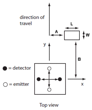
Emitter/sensor board = square with equal length and width = 3.19in / 81.02mm

Entire water tank length = 23in / 584.20mm

Distance from floor to emitter/sensor board = 3.13in / 79.50mm

Distance from center of board to side of water tank = 3.13in / 79.50mm

Aluminum

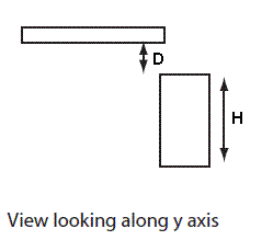
L = 1.25in / 31.69mm

W = 0.58in / 14.76mm

D = 0.36in / 9.15mm

H = 2.77in / 70.29mm

Iron

L = 1.26in / 31.88mm

W = 0.96in / 24.32mm

D = 0.39in / 9.84mm

H = 2.74in / 69.60mm

Acrylic (flipped so that the well is on the bottom facing the floor)

L = 1.26in / 32.00mm

W = 0.99in / 25.10mm

D = 0.80in / 20.54mm

H = 2.33in / 58.9mm

Plastic

L = 1.36in / 34.62mm

W = 0.76in / 19.24mm

D = 0.39in / 9.93mm

H = 2.74in / 69.51mm

Grape on acrylic block

One grape was put in the small well etched on the top face of the acrylic block.

Grapes were approximately 20mm diameter spheres.

D = 0.393in / 10mm

Brass cylinder

Diameter (L and W) = 1.75in / 44.61mm

D = 0.52in / 13.25mm

H = 2.61in / 66.19mm

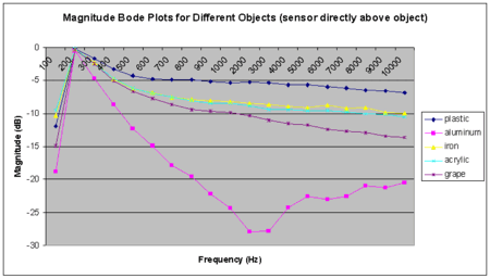
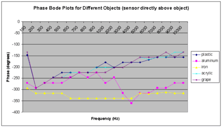
Bode plots for different objects with the sensor directly above the object.

Aluminum seems to have a characteristic response significantly different than the other objects.

For this experiment, all objects were placed in the water tank approximately at these specifications

A = 0.00in / 0.00mm

B = 0.00in / 0.00mm

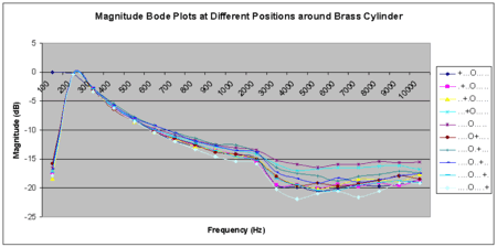
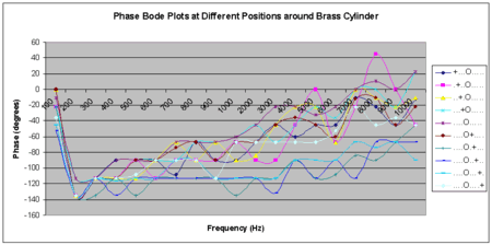
Bode plots as the sensor moves past a brass cylinder

Especially at higher frequencies (4kHz to 10kHz), the magnitude values are the greatest when the sensor is directly above the brass cylinder.

For this experiment, the brass cylinder was placed in the water tank approximately at these specifications

A = 0.00in / 0.00mm

B = 1.48in / 37.60mm

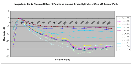
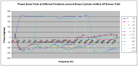
Bode plots as the sensor moves past a brass cylinder shifted off to the side

There is a big jump and plateau for several frequencies in the 3 phase bode plot curves where the sensor is near the object.

For this experiment, the brass cylinder was placed in the water tank approximately at these specifications

A = 0.80in / 20.00mm

B = 4.45in / 113.07mm