Intelligent Oscillation Controller
Team Members
Scott Mcleod: Electrical Engineering Class of 2009
Brett Pihl: Mechanical Engineering Class of 2008
Sandeep Prabhu: Mechanical Engineering Class of 2008
Overview
The overall goal of this project is to create a system that induces a forcing function upon a basic, spring, mass, wall system to achieve an arbitrary periodic acceleration profile (a combination of a 10 and 20 Hz sine wave for our system) on the mass. An accelerometer is mounted upon the mass in the system. A PIC microprocessor records this acceleration data as well as controls a speaker (with the help of a DAC) that provides the external force to the system. This PIC communicates with MATLAB via Serial RS-232 communication. MATLAB processes this data and sends back a control signal for the speaker. After several iterations the actual mass acceleration profile begins to match the chosen profile it is told to "learn."
Mechanics
The basic mechanical system for this device is a simple one, but must be assembled with precision. The major components are the speaker, linear ball bearings on a precision rod, and a spring. First, the speaker is mounted perpendicular to the ground. This must then be attached via a rod to the mass. We tried several approaches, but what seemed to be the best solution was to epoxy about a one inch section of PVC pipe to the center of the speaker. The diameter of the pipe we used matched the diameter of the junction in the speaker where the cone turns from concave to convex. This pipe also had two tapped holes running along the length of the section for a plate to attach to. The plate attached to this PVC also had a threaded hole in the center for the rod that attaches to the mass. The forces exerted by the speaker are small enough (our measurements show only about 3 Newtons) that only about an 8 ounce mass is needed. The bearing we used didn't require any additional mass to satisfy this constraint. The other end of the rod simply attached to the block which we machined and mounted atop the bearing. A piece of sheet metal was screwed into the other side of the block with spacers. This piece of metal is used to anchor spring to the mass, and allows the spring to easily be removed. A similar piece of sheet metal is attached to the wall on the opposite side of the spring. However, this sheet has a vertical slot about an eighth of an inch wide cut from the bottom. This allows the coil of the spring to slide up further on the plate, thereby creating a more solid connection.
It is important to design each component with all other components in mind at the same time. Mainly, making sure that the linear slide is level, and the rod attached to the speaker is centered, level, and in line with the mount on the mass and spring on the opposite side of the mass. This will help to ensure that all motion in the system is one dimensional.
The above was not the first iteration of our mechanical design. We originally had a homemade linear slide. However, we found the lack of precision resulted in unreliable bode plots of the system due to loose tolerances of the design creating side-to-side motion. The first iteration also had the rod epoxied directly to the mass and speaker. During initial testing the connection between the speaker and rod actually severed.
This current design is advantageous because it is modular. The threaded rod allows for minor distance changes to ensure the spring attached to the wall is at its natural rest length. To attach it the plate is detached from the PVC on the speaker and screwed onto the rod. With the spring detached, the other end of the rod is screwed into the threaded hole on the mass. Finally, the plate is then screwed into the PVC through the threaded holes. The non-permanent spring attachment also allows for springs with different k-values to be added to the system. If the spring is longer or shorter then desired, a simple change in rod length is all that is needed to incorporate the new spring into the system.
Circuitry
Programming
PIC Code
In our project, a PIC was used to drive the speaker via its I2C digital-to-analog converter and record accelerometer values at fixed intervals. Since the control system’s algorithm requires too much processing for the PIC, all the computations are performed in Matlab after the accelerometer data is transported to a computer via a serial cable. This setup simplified the program for the PIC.
To generate the waveform of voltage levels sent to the speaker, a single quantized period was used. Since the waveform is periodic in nature, the wave can be repeated indefinitely in a continuous fashion. The nature of our processing algorithm constrained the number of samples for the accelerometer data to be equal to the number of samples for the control voltage.
Since our system used a waveform of fixed intervals, we used an interrupt service routine (ISR) to change the wave and record accelerations at precise intervals. We chose to sample each signal every 1ms (as this is an achievable I2C speed and ISR). To oscillate our system at 10 and 20Hz, we needed at least 100 samples per waveform (1/10Hz / 1ms = 100 samples/waveform). For this reason, we created two 100-byte long vectors for the control voltage ‘u’, and the acceleration data ‘acc’.
Matlab Code
The Matlab code simply follows the protocol as established above. The user specifies in Matlab the parameters for the amplitude and phase of the desired acceleration waveform. *Note that the frequencies of these waves are set to 10 and 20Hz (as constrained by the transfer functions captured from the Bode and the periodic nature of 100 samples/wave).
Below are the 4 m files used in Matlab. Their names must be changed to the last part of their filenames as they are functions.
Main Matlab Loop
Learning Control Algorithm
Smoothing Algorithm
Plot Initialization Code
Program Flow

Control System
To “learn” the control voltages to create a desired waveform, a simple proportional control system was used. We should note much of this code was developed, tested and debugged by Tom Vose, who was invaluable to our final project. Below is our understanding of Tom’s control algorithm.
The system first guesses a control voltage of all zeros. This ideally results in no forcing of the speaker and a flat response of acceleration. After this initial guess, the program uses proportional control to match the desired acceleration waveform. Mathematically, it multiplies the error by a proportional factor k. The error is computed by subtracting the Fast Fourier Transform (fft) of the measured acceleration from the fft of the desired acceleration. This error is multiplied by the proportional control k, and two discrete Bode plot values corresponding to the transfer function of voltage to acceleration at 10 and 20Hz. The resulting signal is the control signal u, in the frequency domain. From here, the control signal is converted back to the time domain via an inverse fft, and sent to the PIC. All of the math is computed in discrete time, for the waveforms of 100 samples long. Below is a block diagram of this control system. Note that it is in the standard unity feedback form.

Results
Below are three tests performed on various superpositions of sin waves at 10 and 20Hz. We have adjusted the phase of the waves to produce different results.
- Matlab Plots Acceleration Desired vs. Experimental Acceleration
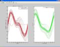
Wave 1
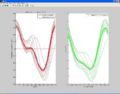
Wave 2
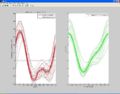
Wave 3


In these diagrams, we are seeing one period of an acceleration profile. The faint blue curve in the left subplot is the desired acceleration motion. The red lines on top of the blue curve are experimental accelerations as recorded by the pic. We can see that the red lines converge on top of the desired blue motion.
Each wave follows the equation below with the given parameters:
acceleration_desired = amp1*sin(2*pi*base_freq*t+phi1) + amp2*sin(2*pi*(2*base_freq)*t+phi2)
Wave 1: phi1 = 1, phi2 = 2 Wave 2: phi1 = 0, phi2 = 0 Wave 3: phi1 = 1, phi2 = 0
Potential Applications
A common question regarding this project is its applications to the real world. In the Northwestern University LIMS lab, a similar type of undertaking is being researched, but on a much grander scale. This same type of oscillation control is being done for 6 dimensions (X, Y, Z, Roll, Pitch, Yaw). However, the microprocessors used in this type of control are extremely expensive, and this one dimensional test of a learning system provides a possibly cheaper solution. The six dimensional control system has possible real-world applications in product assembly.